Michele Oliosi

Hi ! Sorry for the delay as this is a difficult question. As you point out, there is a complex hierarchy of uncertainties, some of which are well-defined, others less so. Just zooming out at first, we tend to classify the relevant uncertainties according to the use that you intend to do. As one goes down in the hierarchy, the order of magnitude of the uncertainties decreases, in general. It is an okay approximation to assume that the uncertainties are compounded with an RMS sum. The first level would be in the case of yield estimates or PXX evaluations. In this case, the dominant factor is: The year-to-year weather variability (O(5%)) The second level is in the case of comparisons with actual data, when you use measurements, or historical data as input. Here the order of magnitude can vary widely, both for the measurement uncertainty, or the parametrization (e.g., given the experience of the modeler). However, certain studies, e.g., the PVPMC blind modeling, show that this uncertainty can be higher than expected ! All in all, I would summarize these uncertainties as (O(1%)). Measurement uncertainty Parametrization uncertainty The third level is the case of tracking the differences between two system choices. For example, deciding between two cable sections. Intrinsic uncertainty of the models. This is the main factor, but each model building block has a different uncertainty. We do not have an exhaustive answer for all models. However, we estimate the base models to have a very low (negligible) uncertainty (O(0.1%)) on the overall results: One-diode model Transposition model DC to AC conversion Ohmic resistance models Some choices of model are more critical, and can yield larger uncertainties. For example, the electrical shadings partition model, in the context of complex shadings, can have a 0.5% uncertainty because many approximations are being made. However, in a context of regular rows it has very low uncertainty. Another example is the central tracker approximation for diffuse shadings, or the sub-hourly clipping effect, which not only yields an uncertainty but also tends to bias the results. Overall, we still need to publish a more exhaustive list (honestly, it is a bit of a daunting task). Conclusion To finish the discussion with a comment more on point on your question, I think that for the purpose of the PXX evaluation, you can entirely neglect the modeling uncertainty. Since the intrinsic model uncertainty is two hierarchies lower than the weather variability, it is probably masked by the uncertainties above. Some exceptions are some critical choices, such as: the partitions electrical shading model in a context of complex shadings, diffuse shading representative tracker approximation in a context with tracker patches, the sub-hourly clipping effect, the bifacial model, any other situation that requires some important approximation that is not adapted to the case studied.

Just a wild guess here, but can your 3D scene support all the changes in plane azimuth and plane tilt ? Indeed, if you change these in a 3D scene, possibly there will be collisions with other shading objects or among PV tables.

Hi, I think that you are not focusing the correct reason for the differences in your loss diagram. Indeed, the effective additional “Global irradiance on rear side” is the same in both cases, i.e., you can expect that the area contributions to the bifacial model are marginal. More important than that is the module area at the stage “Effective irradiation on collectors”. This is not an energy value, so I think the highlighting method in PVsyst failed to see the difference in area. But this is more significant. If there is a difference in area here, it means that the modules have different dimensions in some way, maybe very small. Please carefully compare all parameters of the modules. Also, please make sure that the dimensions of the 3D scene tables have not changed because of that.

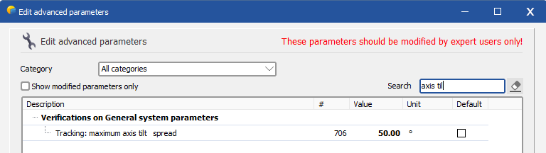
Hi, In PVsyst version 7, this error message is meant to tell you that PVsyst's calculation (which is based on a single average tracker orientation) will have some extra uncertainty given the axis tilt differences in your scene. In future versions, we plan on changing this to a warning, since there are no actionable steps other than removing the trackers that are further from the average. At the moment, we actually recommend to just change the sensitivity threshold for the message. You can easily do this by going to the home page > Settings > Edit advanced parameters. There, you can look for the following parameter: This will let you simulate. By the way, a similar parameter exists for the axis azimuth.

I think that in this case, the expected yearly average degradation of the modules is less than 0.4%/year. I cannot say by how much exactly, but you can try 0.3%/year, which is in the range of what n-type modules have. You can adapt the mismatch degradation accordingly (also 0.3%/year). We do not have information on how the dispersion of the degradation happens for this module, but a reasonable assumption is that it is less extreme if the modules also age less.

In PVsyst the input data is the irradiance. Now, if you use a pyranometer to measure the irradiance and import in PVsyst, the effect of rain will be included. However, any change of IAM due to rainwater is not modeled. Whether the satellite data model for irradiance includes rain effects, this is to be seen.

Sure, you can send the original CSV, the modified Excel sheet, as well as the report, over to support@pvsyst.com. We will look into it.

Hi, It seems excel doesn't read your entries as numbers. Usually numbers are right-justified, i.e., I suspect most entries are read as text or some other type of cell. Please check the cell type, and make sure that all values are actual numbers. Regarding the negative values, it is due to night auxiliary consumption, either from your “Detailed losses” > “Auxiliary losses” definition, or from the inverter definition, or from the transformer night iron losses.

Thanks @dtarin this is a great answer !

No, if the module is marked as “low-light efficiency seems over-evaluated”, it means that the model behaves in an optimistic way in low-light conditions. The message serves to point out that it is “not realistic”.

Dear Dimitri, Thank you for your question. Just a quick reminder, the official language of the forum is English, so you will benefit most from it when asking questions in English (there is no automatic translation). ------- One (difficult to configure) option in your case would be to use monofacial modules of different efficiencies to model the front and the back of the bifacial module. These should be connected in parallel to add up the currents. ------- Another option is to assimilate the bifacial gain to a simpler variant with only a single orientation. Choose only one side of the cross and run the bifacial model. Running the simulation with the backside irradiance modeling on and off will allow you to extract a relative bifacial gain. The perpendicular second side of the cross should be modeled as shading objects (rectangles). Since the bifacial model is not counting the perpendicular side of the cross modeled as shading objects, the shading factor for the backside should be increased accordingly. The proportion of backside shading is likely around 25%. To get a precise idea of the backside shading factor to be applied, you can observe the shading factor for the front side. Then, apply the same shading factor to the backside by means of the parameter in the bifacial model. The mismatch parameter for the backside should also be assimilated to the electrical shading loss of the front side.

Indeed, this hasn't been fixed yet. It is currently planned for version 8.1. There is one workaround I can think of: if the weather data has been imported from a file, you can also import it separately month by month as different files (by splitting the original file by months). This will give you MET files that contain only one month. Simulating with them will limit the simulation to the date range included in these files.

Hello, In the current PVsyst version, there can be only a single tracker orientation at a time, unfortunately. Therefore, splitting in two orientations is indeed the only way. You could average them in a single orientation, but this won't be a good approximation.

Thanks for the feedback. We have a ticket to improve this in version 8. Indeed, the bifacial model window was initially aimed at experimenting with parameters, but it is quite confusing when designing projects.

No, since PVsyst determines the efficiency normalized on the module area, it is necessary to work with the latter for consistency. There is no difference in terms of accuracy, it is more a matter of convention.

Not in version 7, trackers are not compatible with fixed orientations. You need to simulate them separately. In future version 8, this will however indeed be possible.

Indeed, thanks for the answer ! 7.4.6 is correct, i.e., a 2.3 cm imprecision will generally cause shadings shorter than a cell width, by which electrical shading losses are not so critical.

This message is not very explicit, and will be improved in later versions. Basically, either: You use the orientation "unlimited sheds" and put "No shadings" in "Near shadings". The shading loss is already included in the "unlimited sheds" model. You use the orientation "fixed plane" and use a shading model in "Near shadings"

As mentioned, in PVsyst you can only have the power output for a system as a whole. If you need the power output per MPP or per inverter, you should define a system containing only 1 MPP input, or only 1 inverter.

Hi, I don't think that makes sense, in particular for P90. A percentile is a statistical summary value for a given distribution of results. Generating an instance of time-series results that gives a particular summary does not have any significance, i.e., you cannot learn much from this. We can gladly discuss details if you do not agree. The P50 is a bit special because it tells you the average results, and you can assume that aiming for a given P50 may model a “realistic time-series”. However, I am not sure what you can gain from having a P50 time series shown in a table in a report. Analyzing the time series can give you some statistical information on the distribution of results, but you would need some summary values to make sense of that. At the moment, the only way to get a time series to be shown in the report (but only as a list of yearly values, not monthly) is to use the aging tool with previously prepared time series weather data. You can also generate monthly output files from running the time series in the aging tool and make your own formalized output from that.

Dear Shivam, Can you send your project to support@pvsyst.com? We will need to analyze it in details, since it changes only for one of your sub-arrays. Once you send it we will look into it asap.

Hi, Unfortunately, PVsyst can only export variables for the system as a whole. In order to have power losses per MPPT, you need to make different variants with one of the MPPTs only and run the simulation for each of them. This will be very time-consuming, so I wouldn't advise doing it. Same thing for the shade by module, it is not an export value for PVsyst. You need to make a special scene with a single module to get the shading values for a single module. At the moment, in PVsyst, the best in terms of stringing is the single line diagram. However, there is no spatial layout associated with it. You can also print the "Module layout" definitions to color-code the stringing with a spatial layout. However, there is no legend associated to it.

Yes that seems correct !

Could you send the shading scene at support@pvsyst.com ? We could take a look at it. Indeed, 7% electrical shadings seems like too much. I also don't understand why it's 99% shadings and not 100%. Also are you modeling with which version and which shading model (fast or slow)?

This is not simple, but let's see what we can do. First, mutual shadings tend to happen starting with 20°- 30° angles of sun height. These are the times when backtracking is interesting, but also where it seems you are expecting glare. So you have a double constraint on these low sun angles. Note that at times when backtracking is limited, you will have mutual shading. In these cases, it will be best to use just regular tracking. This is because backtracking is only convenient whenever you are removing most of the mutual shading (and electrical mismatch effects). So once you are in a mutual shading regime, I think it is probable that regular tracking will be best. Based on that, you can run two simulations: one with backtracking and one without. For each of them, you can generate an hourly output file. Then you can process the data, and use the regular tracking one whenever the backtracking rotation angle would be < 20°. The resulting dataset can then be summarized to obtain yearly yields, etc.