-
Posts
897 -
Joined
-
Last visited
Everything posted by dtarin
-
Have you tried creating a copy of the SIT file in the Sites folder, to see if it shows up in the list?
-

Energy Generation Difference between Report and Aging Table
dtarin replied to Solaranger's topic in Problems / Bugs
I am seeing difference of 0.15% in 8.0.12 which is non-trivial. Aging tool on top, PVsyst report result on bottom. -
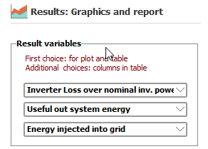
Useful Out and Egrid are the same. I suggest including InvOut It seems IL Pmax will include grid limitation loss when there is a limit applied in the IL Pmax figure, even if it is set to account for loss separately under energy management. I suggest quantifying IL Pmax as its defined in energy management, or by default include POI loss as a separate value, and let users add together if they want. EArrayMPP is more useful than EArray, I recommend adding it or replacing EArray with it.
-
PVsyst doesn't output 8760 files past year 36. It will complete the simulations and generate the pdf report, but not the excel output. v8.0.12
-
Simulate with as few trees as possible. Take into account things like the total elevation at the top of the trees (tree height + ground elevation) and the distance relative to the panels.
-
export simulations to excel. output the variables you need and analyze from there.
- 7 replies
-
- shadings
- shading scene
-
(and 1 more)
Tagged with:
-
Losses due to specific objects are not isolated. Shading from turbines will be included in both near shadings and electrical loss in the loss diagram. To isolate the turbines run models with and without them, take the delta of shading losses and you can calculate whatever you need. You will also have energy with this, so you can easily calculate overall energy impact monthly, etc.
- 7 replies
-
- shadings
- shading scene
-
(and 1 more)
Tagged with:
-
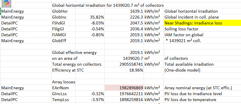
EarrNom and all resulting energy are not shown correctly when exporting loss diagram values from the report. The report itself is correct, but the exported values are not.
-
The 1100UD is one inverter module that is typically installed with other modules in a single PCS, like the 4400UD-MV. You will have four mppts with the 4400, each 1100 is one mppt as stated above.
-
If it still doesn't work you can always model it as I have above 🙂 The gaps will not matter for bifacial calculations, they are not used. The user defines the transparency factor manually which takes into account gaps in structure, modules, etc. So I'd either model as I have or increase the gap in your method if the suggestion above does not work.
-
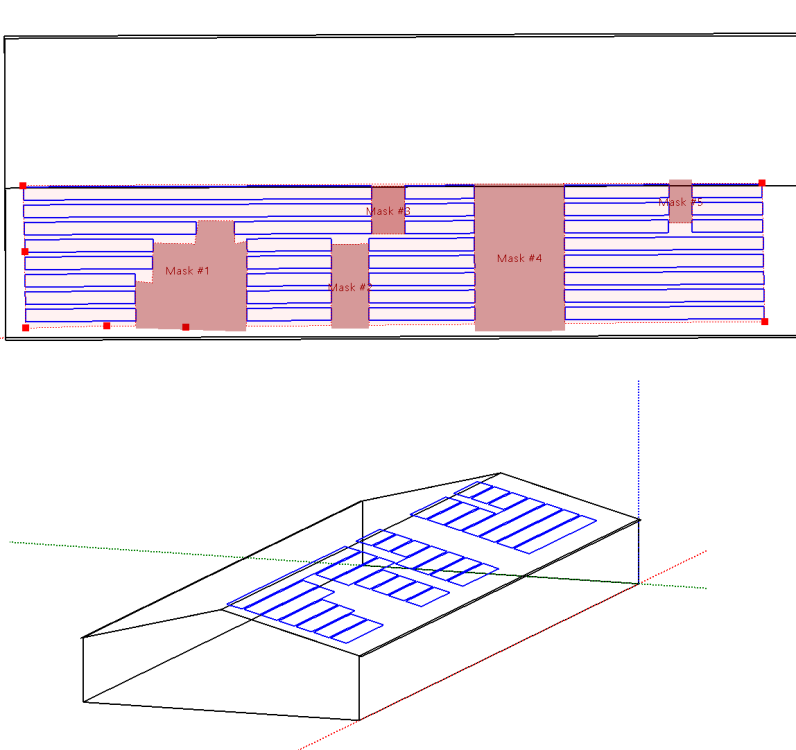
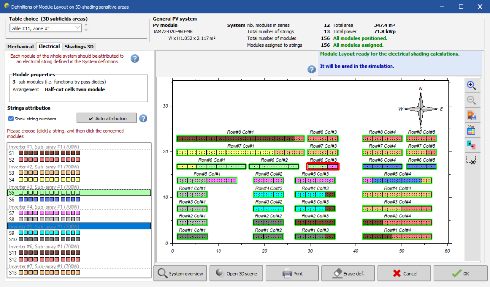
I don't have any the details of this system and haven't modeled solar edge in a long time. However, with a zone you can auto set table to fill the zone, auto tilt to adapt to slope of roof, set table size to 1x1, and then use module layout for allocation (electrical loss). Keep in mind this is just for shading calculation, not power, so you don't need it perfect. As long as it is reasonably close to capturing the shading conditions it should be fine. You create a single zone, insert masks, auto fill the zone as shown. This will allow you to model bifaciality.
-
OND files are for inverters. It is typical to receive from manufacturer if it is not listed in database already.
-
Modifying the OND file is another way
-
While that is being investigated, in the past, these types of issues were caused by the default program assumptions overriding the project settings. The default value is 0.02. In the main PVsyst menu under advanced settings, set the default to 0.00 or 0.01. Import your shade scene where things are showing up correct, save, and reopen to check. The warning about tables not defined by modules is not material in most cases.
-
Reduce the size of the window then maximize again.
-
The inquiry above is related to the inquiry here, which is the slope (tilt) of the table does not follow terrain, only the elevation.
-

Medium voltage line + medium voltage external transformer
dtarin replied to arnaud pancrazi's topic in Simulations
Total loss -
The first section for AC loss should be zero. The MV AC losses are further below, they will not be zero. There is no good way to model it. Modeling with 1 overestimates loss, modeling with 2 underestimates loss. For an in-between figure you can simulate with 1 partition and again with 2, average those and calculate energy delta from your base case, then apply that delta in a new simulation in MQF. For example, base case A is 1 partition, case B is 2 partitions. The two partitions will likely have higher energy. Then calculate (EArrMpp_B - EArrMpp_A) / (2 * EArrMpp_A) and include this result in MQF in a new simulation for case A.
