
dtarin
-
Posts
897 -
Joined
-
Last visited
Everything posted by dtarin
-
Why not adjust the bifacial albedo to 0.7? If this reflector is not flat on the ground, maybe Sunsolve can simulate it.
-
If bifacial is disabled, the variables will not be available, same for the horizon loss.
-
DiffGnd definition missing from documentation.
-
You can download time-series data (20+ years) from https://nsrdb.nrel.gov/data-viewer. From there you can calculate it manually from GHI or import each year into PVsyst. You can also get ~18 years of data at PVGIS free https://re.jrc.ec.europa.eu/pvg_tools/en/#MR.
-

Generating an output file for later years using the aging tool.
dtarin replied to Tonderai's topic in Simulations
Go to output file, check the box "file name" under "output file". Set your variables. The name doesnt matter. Hit okay. Go to aging tool, have your ageing parameters set, I check both output file and report (to see everything ran correctly), click run simulation from within the ageing menu. it should output then. -
Why are diffuse integrals calculated for every run?
dtarin replied to LauraH's topic in Shadings and tracking
It would be helpful to include this in the next update. We've had to use custom tracker approximations to avoid long waits for diffuse recalculations when making other unrelated model updates. -
Multi-Year Analysis of Inverter Clipping Losses & Module Degradation
dtarin replied to ASZulu's topic in Simulations
It is expected for plant/inverter clipping to decrease as system capacity degrades. -
Bumping this. Any plans to incorporate this in future versions? Modern design software spit out shd or pvc files quite easily (both should be able to be imported). I think the only hangup with this is the partition definition for each shade scene, but if this were added to 3D shadings parameter, the user could define the geometric area of a partition that gets applied to each scene. Diffuse shading can be set to central tracker for quick analysis by default, backtracking activation is already an option for batch sims.
-
How to configure a tracker to lock the rotation
dtarin replied to Antonio Augusto Ananias's topic in Simulations
Curious why you have included the +1 there. You can simulate a tracking system at [X,X] for min and max to lock the tracker for all hours to a single angle. If you need to more than one angle, this can be done with batch simulation easily. -
Tracker Power Supply Demand - Where to mention?
dtarin replied to Job Sebastian's topic in Shadings and tracking
Auxiliaries tab: proportional to inverter output power (i.e., 1 W/kW = 0.1%, etc.). -
If the sensor(s) is in front of the torque tube and other items, (GlobBak+BackShd) * 𝜑 is sometimes used. Install sensors midpoint between two piles for tracker systems.
-
Ohmic loss is proportional to power. Abu Dhabi has much higher irradiance compared to Berlin. Also, not sure if it is intentional, but you're simulating the 10th year of operation. If unintended, be sure to set it to year 1 on the degradation tab. Ohmic losses - PVsyst documentation
-
This looks like an AI bot or something...
-
Still present in 8.0.16, don't see mention of correction in 8.0.17 or 8.0.18 release notes.
-
You are modeling "detailed according to module layout". You need to place these modules in the tables in the module layout menu. Select "according to module strings" and it will use the shade scene as it has been provided. The total area of the shade scene is relatively close to the pv system.
-
After writing that, perhaps the issue is that your prj file itself is missing the .SIT information, in which case manual creation might be the solution.
-
You can always create one from notepad just to get it loaded or extract the site information from the .prj file. Look for the following (and remove the text after the underscore). Some changes will need to be made; I think you just need to add the version below the "Comment=..." line. If you're creating from scratch, I think the main things you need are coordinates, altitude, timezone. The meteo data that is contained in the site file is not used in simulation. PVObject_SitePrj=pvSite .... .... End of PVObject pvSite
-
Hello, It would be great if we could specify .SHD files in batch simulations.
-
Will the Perez-Driesse model be included as an option in the future?
-
Export the data (values) from the graphs and you will get short circuit values for V and I.
-
Electrical shading loss has been around for a long time. It is likely the 7.2 report was run on linear shading, or the site was modeled perfectly flat with backtracking enabled and no shading objects present to cause electrical shading loss.
-
Representation of gaps along tracker when using PVcase scenes
dtarin replied to LauraH's topic in Shadings and tracking
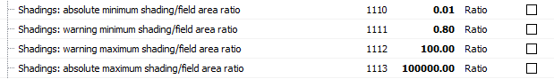
You can change the settings for both types of messages. The shade scene module count has no impact on simulation results.
-
Partition Definition in 3D Scene with 2-Portrait Trackers
dtarin replied to Alessia's topic in Shadings and tracking
2x28 = 4 vertical, 1 horizontal for half-cell module -
norm.inv(Pxx,0,1). P99 is 2.33, not 2.35
-
Cannot get custom tracker to save in v8.0.12. Once shade scene is exited, it remains all trackers.