-
Posts
2075 -
Joined
-
Last visited
Everything posted by André Mermoud
-
If you have a multi-MPPT inverter, no problem, you can define a sub-array per MPPT input. If it is on one only MPPT input, it is not possible in PVsyst.
-
For usual meteo data, the "official" altitude according to WMO standards is 10m, without surrouding obstacles. Now in PVsyst, if you have values measured for instance at the array level (or 1m above), the velocity values are about 30 to 40% lower, so that the Uv parameter should be increased by this amount.
-
Yes, PVsyst includes the Meteonorm and the NASA-SSE data, for anywhere on the earth. Please see our FAQ Which meteo data are available in PVsyst ?
-
If the module is not in the database, it can have been defined by the mentioned third-party. - Either you got the project as PVsyst source (PRJ and VCi files). If the sender has exported the project by "Files" / "Export projects", the PAN file should be in the project's data. - If not, you don't have any mean of recovering this file. You should redefine this module (PAN file) from Datasheets information, and you are not ensured that the "uncertain" parameters like Rserie and Rshunt are the same.
-

Multiple module Mix in same inverter
André Mermoud replied to Shilpidangi's topic in Problems / Bugs
I can't understand that. Please send your full project (using "Files" / "Export projects") to support@pvsyst.com. -
The batch is meant for analysis and comparison of several executions one with respect to the another one, and for any specified variable. There are hundreds of ways using this functionnality. I really don't see how to present a meaningful report.
-

Multiple PV Modules with our Inverter configuration
André Mermoud replied to purnaanshg's topic in How-to
This configuration is not possible with PVsyst. The master/slave functionnality is only useable within one given sub-array. This limitation is quite understandable: if you connect your inverters in Master/Slave mode, all the PV sub-arrays will be connected together as a same array. PVsyst (and the best practices of PV) cannot manage heterogeneous arrays, i.e. array with different modules and/or different numbers of modules in series. Be careful with your strings of 20 Trina and 18 Renesola modules in parallel: the operating voltages will not be the same, you will have a significant mismatch, and you can get double Maximum power points, with the risk that the inverter chooses the lower one. -
As I asked after the previous question, please send me this MET file at support@pvsyst.com
-

Multiple module Mix in same inverter
André Mermoud replied to Shilpidangi's topic in Problems / Bugs
This is the right way: on a given sub-array, you can only define homogeneous arrays (i.e. same PV module model, same number of modules in series). Now if you define an "normal" inverter with 2 MPPT, the report will mention one inverter and 2 MPPT. In this case the 2 MPPT inputs will be considered as 2 identical half-inverters In your case you have specified "with unbalanced inputs", I don't know why. This is a very special case (suited for special inverters). With this option the MPPT inputs are specified as "Main" and "Secondary" input. In your system definition you have to define a sub-array for each of these inputs. If you define 2 "Main" inputs, this will mean 2 different inverters. -
The choice of a project or a meteo file may become slow when the list is long, i.e a common list of projects shared by many people. Because each file of the directory has to be open for extracting information for the list. And this is still made worse if the access is through a network. However this reading is normally done once only for each run of the software. A solution could be to remove the old projects or meteo files (no more in use), i.e. to store them in an archiving data structure. In "Files" / "Workspace", you have the opportunity of easily switch to another data structure.
-
The Uc and Uv parameters are not related to the location nor climate, but the mounting mode of the modules (if they are integrated - i.e. back insulated - or not). Now we don't have really well assessed values for these parameters. Please see the Help, available by F1 when you are in the U-definition dialog.
-

Several Orientations - Global on collector plane
André Mermoud replied to avielk's topic in Problems / Bugs
This is indeed a bug: I have forgotten updating these 3 labels (Transposition FT, Loss and Global on coll. plane) in the multi-orientation panel. I have corrected for the next version 6.27, to be released within 2-3 weeks. However these are just values shown as information when choosing an orientation: these are not used anywhere in the simulation. -

Difference between Pvsyst and NREL's Solar Position Algorithm
André Mermoud replied to bertin's topic in Simulations
I don't know, I have never implemented the NREL algorithms. The fact that the differences are rather "symmetrical" around 12H indicate that the problem is probably related to the time definition. The sun progresses by 15°/hour (along its trajectory). Therefore a discrepancy of 3° in the morning may correspond to a very high time discrepancy (3°/15° corresponds to 12 minutes, to be divided by cos(slope of the trajectory at sunrise) ). However in subtropical geometry (trajectory almost "vertical"), I don't understand well how you can get 3 to 5° error at sunrise. The problem of the accuracy will mainly arise if you perform a retro-transposition for getting the GHI and DHI from a measured DNI value. The morning DNI calculated from the GHI and DHI may have a significant error, but without consequence on the incident irradiance on your almost horizontal plane. PVsyst provides the opportunity of specifying a time shift, already at the meteo data import time, which can avoid this problem. -
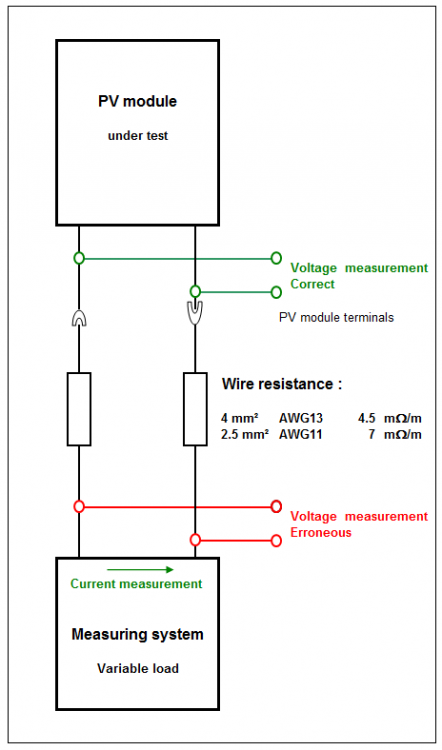
The IEC 61853-1 standard now recommends the measurement of the PV module characteristics under a matrix of different irradiances and temperatures (namely 1100, 1000, 800, 600, 400, 200 and 100 W/m2, for temperatures from 15°C up to 75°C). The low-light efficiency is the basis for the determination of the uncertain parameters of the one-diode model in PVsyst, mainly the Rserie value. These measurements should be performed with high quality flash-test instruments (AAA class). The irradiance attenuation is ensured by calibrated filters. The results are usually provided as ( Imp, Vmp, Isc, Voc ) data sets, for each (Irradiance, Temperature) condition. Let's define: - PmpMeas = Imp * Vmp measured at GMeas = nominal irradiance after filter - PmpSTC = Imp * Vmp measured at GSTC (= 1000 W/m²). The relative efficiency is then (PmpMeas / GMeas) / (PmppSTC / GSTC) - 1 Filter uncertainties One problem is that the filters are not perfect. They may have inaccuracies either in irradiance and in spectral response. Then, an error of 1 % on the irradiance means an error of around 1% on the relative efficiency. For avoiding this problem we can follow the hypothesis that the short circuit current is proportionnal to the irradiance (including spectral mismatch). From experimental basis, this hypothesis is proposed by the Sandia National Laboratories (USA), as a direct measurement of the incident irradiance. In the "theory", it is the basic hypothesis of the one-diode model. During the analysis of the low-light data, a correct estimation of the relative efficiency requires to modify the GMeas nominal response of the filter by using a corrected irradiance GmeasCorr = IscMeas * GSTC / IscSTC Electrical measurement setup Another key point of the measurement of low-light efficiencies is the electrical measurement of the voltage: this should be measured as close as possible of the PV module terminals (so-called "four-wire" measurement). If the voltage is measured at the measurement instrumentation level, the cable resistance will add with the Rserie of the module. As an example, if you have 2 x 5 m of 4mm2 cable (AWG 11), the parasitic resistance will be of 45 mOhm. For a usual 250 Wp modules of 60 cells, this has to be compared to the Rs = 310 mOhm. The addition of this parasitic resistance will induce an error in the modelled low-light efficiency of +0.33% at 800 W/m², +0.69% at 600 W/m², +1.11% at 400 W/m², +1.58% at 200 W/m². These errors are very important, when we usually see (wait) over-efficiencies between +0.3 and max. +1% in the 600 - 800 W/m² range. NB: The current measurement is not affected by voltage drops due to parasitic resistances. Four-wire voltage measurement
-

Creating Measured Data Analysis Variant
André Mermoud replied to vrajeshpatel's topic in Problems / Bugs
Passing from a "normal" calculation version to a comparison calculation is not simple. However we will probably deeply review the Measure-simulation Comparison tool within some months, and I put this suggestion as a topic on which we should pay attention. -
PVsyst is not meant for the full study of the grid organization after the PV system, which may take many different forms (one or several transfos or voltages, etc). There are probably specialized software for that. However we wil probably think about this suggestion after our present numerous development priorities.
-

How to Correctly Simulate a Horizontal SAT w/ Fixed Tilt
André Mermoud replied to Paul G's topic in Shadings and tracking
I already answered: you have to use the tracking frame, with a fixed tilt for the tracker. Now there is no differences in the algorithms, it is always the Transposition model (Hay or Perez). But the "physical" plane orientation is different in both cases. -
This is not yet possible. The losses defined in stand-alone systems are restricted in the present time. I will update this treatment during the next few months.
-
You can have a look on our FAQ How is defined the plane orientation?
-
SMA has not proposed the data for the OND files corresponding to this model for the PVsyst cdatabase.
-
Nothing has been changed since the beginning of version 6. The update works quite well. However the problem may be some change in your web access. Some proxies or special web access right restrictions may affect the AutoUpdate possibility.
-
The simulation button is grayed because you have a red warning in the sizing form ("The array is strongly oversized"). Please see the FAQ Can I define a system with highly undersized inverter ?
-

Simulate 1 minute power output based on measured 1 second data
André Mermoud replied to aarabi's topic in Simulations
Sorry, PVsyst only works with Hourly data. It is not able to perform simulations on sub-hourly intervals. -
These values are the same if you don't specify Soiling losses. The soiling losses will also be taken into account in the GlobEff value (it is the effective irradiance in the PV modules).


