

Michele Oliosi
-
Posts
763 -
Joined
-
Last visited
Posts posted by Michele Oliosi
-
-
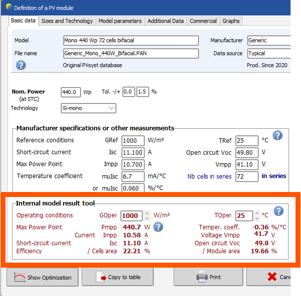
BNPI conditions cannot be used as input in PVsyst. You could use the BNPI test report to re-evaluate the bifaciality factor. But per se the BNPI result will not be used in the simulation (in which irradiance and temperature conditions vary at every step).
To calculate the bifaciality factor the approach would be as follows. The basic equation is Pmeas(BNPI) = P(1000+phi * 135), and solve for phi (bifaciality factor). This could be solved by trial and error using the PAN file interface to evaluate P(irradiance, 25°C), but it will involve manual steps. Once you find which irradiance yields P(BNPI), you can easily find phi.

-
Yes, actually the irradiance of front side + backside*bifaciality factor are put together, which gives an effective irradiance evaluation. Only after that, the PV conversion model applies. Indeed, the light reaches the same cells, be it from the front or the back. The same low-light performance is therefore taken into account for front and back (up to the bifaciality factor).
-
Regularity is defined vaguely by PVsyst. If the system is approximately regular, e.g., patches of trackers or tables that are more or less evenly spaced, then this can be considered “regular” in the PVsyst sense. In that case, you can use the 2D bifacial model jointly with the 3D scene.
PVsyst will check the following points:
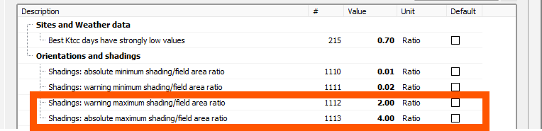
- The RMSD of the pitch distribution. If the RMSD is too large, PVsyst will throw an error. You can change the threshold of the error in the advanced parameters.
- Whether the tables are the same height. If there are differently tall tables, PVsyst will throw an error.
- Whether orientations have more than 2 rows. If there is only one row of tables, PVsyst will throw an error.
- The average axis tilt of the trackers in each tracker orientation. If the average axis tilt is too large, PVsyst will throw an error. You can change the threshold of the error in the advanced parameters.
-
Currently, the rear-side model of irradiance is two-dimensional (cross-section). However, it is compatible with a 3D drawing.
If you have a 3D drawing with a regular arrangement of tables, you can activate the 2D bifacial model to compute the rear side irradiance.
-
Automatic mode will select the tracker with the highest GCR as reference. It is an alternative way to select the tracker pair.
If you deselect the tracker pair, the parameters shown in Pitch, collector width, etc. can be manually adjusted.
-
This is a bug, I have created a ticket to address it.
In past versions, it used to be present in the report.
-
Sorry, this warning is not appropriate in your setting, we still need to address the way it is triggered so that it becomes more relevant.
I think it was added with the case of different nominal orientations in mind. But currently, for your case, i.e., one nominal orientation with many variations due to the topography, the way to go is: use only one orientation.
This has one drawback: the averaging error and the mismatch caused by the individual orientations are not taken into account, i.e., on this end the calculation is a bit optimistic. But since our calculation is already conservative in other ways (e.g., backtracking modeling), I do not think this small underestimation of losses is critical.
In the future, we want to account for these two losses we are yet missing.
-
Hi @Cole Noble,
If you import hourly GHI data into PVsyst meteonorm or DirInt are not used for DHI. Instead, the Erbs model is used.
However, the meteonorm generation is likely used for the ambient temperature if it is not present in your data? -
Hi @tommm, no indeed, as you have understood, there is no way to organize per inverters in this interface.
However, the solution you hinted at should work. I.e., you can define different inverters and open the window “Multi-orientation daily sharing” from sub-arrays with the three different inverters respectively. Make sure everything is checked.
-
Dear Sofia,
Yes indeed, this is a bug we have in the current version. The bifacial model does not handle 0° tilts anymore.
This will be fixed in the next patch 8.0.14. Sorry for the inconvenience..
-
Hi, you need to enter the 3D scene and modify your PV objects to define partitions on them.
Here is a help page with some guidelines on this: https://www.pvsyst.com/help/project-design/shadings/electrical-shadings-module-strings/partition-in-strings-of-modules.html
-
Hi,
This is an order of magnitude estimate, so we did not feel the need to be too precise. To be on the safe side: you can work with twice the distance from the center of the PV site to the edge.
-
Yes, that is also another option, especially since you have a ready-to-use MEF file. 🙂
To address the original issue:
- There was an issue with the units and multipliers, which were not defined correctly. This fixed the error of the clearness index.
-
Hi,
It was indeed possible to define situations with only a single row + 3D scene + bifacial model in previous patches. However, this was not the intended behavior and was a possibility that was exposed by a bug. We would not be able to guarantee that the calculations were properly handled in this situation.
We have recently corrected some issues in terms of number of rows, and that has had the effect that the above unwanted exposure was corrected as well. Currently, the calculation with a single row in an orientation (such as your orientations 2, 3, 4, and 5) can only natively be realized with an unlimited orientation.
There are therefore two workarounds:
- Model orientations 2-5 as unlimited orientations with one row.
-
Duplicate the 3D tables from orientations 2-5 and any objects that may shade them. The duplicates should be placed far enough on the scene so that there are no unwanted interactions. In this way, PVsyst recognizes two rows instead of one. Since they are sufficiently spaced, mutual shading effects are negligible.
-
You may need to alter the following advanced parameters (Home window > Settings > Edit advanced parameters) to avoid some problems with a larger scene than the modules defined in the system window
- This solution does not work with Module Layout definitions (because these necessitate a perfect match between 3D scene and system)
-
You may need to alter the following advanced parameters (Home window > Settings > Edit advanced parameters) to avoid some problems with a larger scene than the modules defined in the system window
Please note that supporting 1 row bifacial orientations is in our internal roadmap, and I will rebound on your request with discsssions to see whether we can anticipate this feature a little.
-
Hello !
Regarding the snow data, actually the snow depth time series data is not used by the simulation in PVsyst. Instead, the impact of snow is present via the albedo factor (monthly). Typically, if snow is present on the ground, the albedo factor is between 0.4 and 0.8. You could check how many days are snowy in a given month, and proportionally increase the albedo.
For the warning on the clearness data, we would need to take a look at the data. Can you send the data and MEF file to support@pvsyst.com? Else, you can share a screenshot of "Best clear days Ktcs" graph and "Monthly best clear days"? That will also help.
-
This is a good remark, it will be useful for many users.
In principle, we do recommend trying to group orientations into fewer average orientations. Usually, orientations should fall into an average whenever there are identical nominal orientations (for example, despite the irregularities caused by a complex terrain), or when they fall into the same DC array, which will facilitate the “System” window definitions.
When there are notable differences, such as different ground types, backtracking parameters, types of racking, etc. it may be worth keeping separate orientations, of course. This will facilitate definitions. For example, if there are different ground types, determining albedo values for each of them makes sense.
However, the default behavior when importing a 3D drawing is not fully in tune with these recommendations, yet. Indeed, by default, the 3D import will separate orientations based on effective angles. Therefore, a necessary step is to regroup orientations. The simplest way is to select all concerned PV tables in the 3D scene, and then use the right-click menu to create an orientation from the selection. Any other method works here, as long as it allows for an educated grouping of orientations.
We are looking into improving this default behavior at the stage of 3D import. Ideally, we want this experience to be more in line with our recommendation of grouping orientations.
-
PVsyst usually takes the minimum pitch as default value for the backtracking algorithm. If only one of your trackers has a pitch of 6.24 this may explain what you observe.
Note that you can anyway override the backtracking parameters from the 3D scene > Tools menu > Backtracking management. -
Two corrections impacting electrical shading results
Release note:
- Shadings: the bottom cell size is now taken into account also when computing the shading factor table from the Near shadings window.
Between versions 8.0.0 and 8.0.11, the bottom cell width was not available in the Near shadings window calculations. Therefore, recomputing the shading factor tables by clicking the “Recompute” button, or computing the tables when prompted when closing the Near shadings window could lead to slightly incorrect results, especially for low sun heights.
Version 8.0.13 corrects this bug. Shading factor table calculations will be consistent no matter where they were called from. If you were using the "according to module strings" model in "Fast", it is possible that electrical shadings will slightly increase due to this correction.
Release note:
- Shadings, thin objects: the partition model results in presence of thin objects have been corrected. This may impact the simulation results, by increasing the electrical shadings slightly in some cases.
In previous patches of PVsyst 8, the electrical shading factor in the presence of thin objects, when using the fast simulation mode (table interpolation), was not calculated correctly. This could lead to an underestimate of electrical shading losses. Note that this bug was not present in version 7.
Moreover (also in previous PVsyst versions), whenever the total irradiance loss was lower than the electrical shading loss from normal objects (case with many thin objects), the electrical shading loss could also be underestimated. Although very rare, this case is now corrected as well.
Improvements of the bifacial view factor model
Release note:
- Bifacial: corrected calculation of the sky diffuse contribution on the rear side of the PV modules
This patch addresses several issues in the modeling of the sky diffuse on the rear side.
- The impact of the number of rows has been reassessed; it now better captures the fact that the rows at the extreme end of the array do not experience mutual shadings, for all diffuse components.
- The rear side diffuse view factor has been revised; a normalization factor now correctly depends on the tilt.
- A discretization effect that caused an East-West asymmetry for trackers has been fixed.
These issues were most impactful in the following two cases: systems with vertical tables, and systems with few rows of tables. With this correction, the modeling of irradiance on the front and on the rear have been harmonized and generally have a better match. However, the impact on the total system output remains small, amounting to less than 0.5% for most bifacial systems.
Note: Systems with a single table, or a single row of tables, can currently only be designed with “unlimited” orientations. A workaround duplicate all the elements in your 3D scene and place it sufficiently far away so that mutual shading effects are negligible.
Considering the power factor in the System window for sizing assistance
Release note:
- System design: Overload losses are now adjusted when a Power Factor is specified in “Energy Management”.
When requesting an inverter to produce reactive power, its overload conditions may be impacted. This will depend on its nominal power specifications.
If the nominal power (PNom) is specified as apparent power ([kVA]), a power limitation will apply in terms of active power according to the formula: PNom(active) [kW] = PNom(apparent) [kVA] × cos(φ).
Since PNom(active) is lower than PNom(apparent), overload losses increase and depend on the chosen power factor (cos(φ)). Once a yearly power factor is specified, the estimation of overload losses in both the System and Sizing windows will take this effect into account, indicated as “Overload loss, with PF”. This estimation now more closely reflects the values shown in the loss diagram.
Future versions will include the estimation of overload losses for monthly power factor as well.
A more detailed explanation is available in the Help section: https://www.pvsyst.com/help/project-design/grid-connected-system-definition/power-factor/index.html
Warning message “inverter is slightly/strongly undersized”
Release note:
- System Sizing: warning and error messages for inverter slightly and strongly undersized are now triggered at 2% and 4% overload losses, respectively. These errors are not fatal anymore.
In addition to the previous point (considering the power factor in the System window), the fatal error message “the inverter is strongly undersized” is no longer triggered at 3% overload loss. Instead, it is now issued as a warning that does not block the simulation.
For new projects, the threshold for displaying this message has been updated to 4%, acknowledging that moderate inverter overloading has become a common practice. For older projects, the threshold is still set at 3%, which can be modified in the parameters of the project.
-
@Pete if you can send the zipped project (Export button in the project window) as well as your result tables (including the batch results file if you used the batch) to the email address support@pvsyst.com
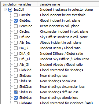
As usual with these investigations, comparing intermediate variables and not just the final energy gives good results in pinpointing the main effect. If ShdDLss is not the issue, then we should look at other variables before and after this point, to see if the energy increase is due to a specific loss or gain along the loss tree.
-
Hi, I would suggest looking at more variables. I strongly suspect that the dominant loss factor is the losses on the diffuse component. These will have a less sharp decrease than other losses, especially in the case of backtracking, which zeroes-out the direct shading losses.
You can take a look at ShdDLss and ShdALss.
-
Dear Ishan,
Real sorry, your question is taking some time to answer. Unfortunately, there are some details that need to be understood. We are trying to provide as informed an answer as possible.We should be able to reply by the end of the week.
-
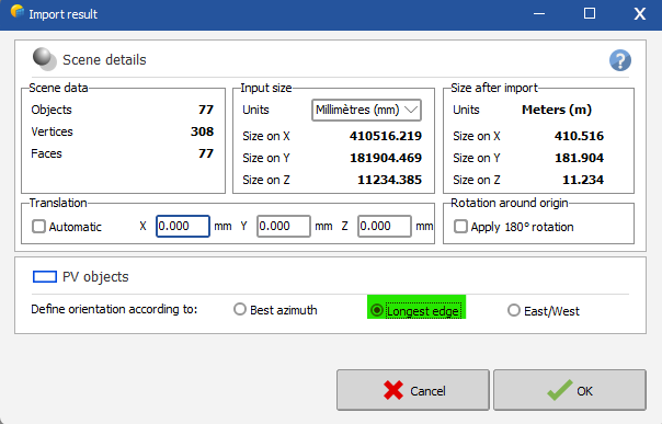
When importing, you should have multiple choices to define the orientation:
Can you try "longest edge" ?
-
The issue of reflection is that it is not explicitly modeled by PVsyst (currently). You should therefore find an indirect way to estimate it, or, better, find another tool that is more adapted.
Also you interested in the reflection as a directional quantity? (for the purposes of glare regulations, for example). Or is are you interested in the amount of light “lost” to reflection, as a way to understand the energy flows?
-
@Leticia Currently, albedo is still stored in the weather file as monthly coefficients. This means that the time series will be summarized into monthly values. The hourly time series will be exploited in a later patch.
These coefficients can then be used in the project settings, but it still requires going to the project settings and click on the button to copy the values from the MET file.
Since these coefficients can end up in the project settings, they are currently intended to be used for the far albedo.
Correct selection of simulation variables for vertical bifacial PV
in Simulations
Posted
UPDATE and correction to the previous answer.
BeamInc + CircInc + DifSInc + ReflFrt + AlbInc/2 + ( - HrzBLss - HrzCLss - HrzDLss - HrzALss/2)
I would suggest now
BeamInc + CircInc + DifSInc + ReflFrt/2 + AlbInc/2 + ( - HrzBLss - HrzCLss - HrzDLss - HrzALss/2)