
André Mermoud
-
Posts
2075 -
Joined
-
Last visited
Everything posted by André Mermoud
-
Yes of course. The best way is to open an existing (similar) module, and change the main parameters (STC values, Number of cells in series, sizes). All other parameters may be let at their default value (check the corresponding checkboxes). Finally save the PV module with a new filename, this will create a new module in your database. You can have a look on the FAQ: How to establish the PAN files?
-
The shed object is a "stiff" object: it cannot be adapted to a terrain. You should define your system as independent "tables". These tables may follow the terrain (base slope).
-
This value is simply the Pnom array, multiplied by the efficiency of the inverter at this power. This is not a very sensitive value. In a future version (not the next one), we will change this way of estimationg the Transformer losses and propose a more understandable procedure based on "real" transformers properties.
-
You can simply suppress all the losses after the inverter (AC and external transformer) in the simulation.
-
 When you elaborate a 3D shading scene, and exit the editor, PVsyst will check that your scene is compatible with the other parts of the system. In particular, it will check that you have defined a sufficient active area (3D fields) in the 3D scene for positioning all modules defined in the "System" part (Subarrays area = sum of the areas of all modules). You can define a greater area in the 3D scene, as your modules may not be completely jointive, but not a smaller one. The match should be satisfied for each orientation. This screen shows the effective areas defined in the System and the shadings part. If you need more details you can find them with the button "System Overview".
 -
The "Warranty efficiency curve" of most PV module's manufacturers show a warranty beginning with 97 or 98% guaranteed efficiency for the first year. In PVsyst, for one module this initial performance loss is mainly represented by the LID losses, which is a real degradation occuring within the first hours of exposure of the PV modules to the sun. There may also be a contribution of the Power tolerance, or you may want to take the Flash-test accuracy (not better than 2-3%) into account. Please ask the manufacturer for this interpretation. The option "Module quality loss" is more suited for taking this initial uncertainty into account. The LID loss or Module quality loss are applied to any simulation, for any year: the PV modules are "damaged" at the beginning, and stay like this all over the system's life. Parameters of the Ageing Tool Please note that the manufacturer's curve gives a Warranty for one module. It doesn't mean that the degradation of all modules will behave in this way. The average degradation for the whole system (average of the modules) will probably be much lower (this was reported as about -0.3% to -0.4%/year, by the very few studies about long-term degradation, and for very old modules). As all the modules will not degrade in the same way, the degradation loss will also be affected by the increasing mismatch between modules along years, which you can model in this tool, using a Monte-Carlo stochastic method. Simulations Simulation without specifying an ageing degradation: this "usual" simulation will represent the system's state at the commissioning time. It includes the initial LID loss. Simulation with ageing, for the first year of operation: this will also include the specified initial LID loss. If you specify a degradation rate of, say, 0.4%/year, then at the beginning of the year the degradation will be null, and at the end it will be 0.4%, therefore an average of 0.2% for the global simulation of the first year. The tool "Degradation" in the detailed losses gives the opportunity of performing the simulation for any given year after commissioning. In the "Detailed Simulation" option, you can perform a simulation over all (or several chosen) years, in order to get a summary of the yield of your system along its lifetime.
-
Unable to import SolarGIS .CSV file in PVsyst6.47
André Mermoud replied to astha.saxena542's topic in Meteo data
Please send us this SolarGIS file (to support@pvsyst.com) -
Tables not interacting with imported ground profile
André Mermoud replied to Brian S's topic in Problems / Bugs
This has been corrected. Please update to a more recent version. -
Array Temperatur differs between simulation runs
André Mermoud replied to Gerd Schroeder's topic in Problems / Bugs
I don't know. Please send us (support@pvsyst.com) the whole project (using "Files > Export projects"), and explain exactly where and how you find this problem. -
Sorry. This has been corrected (and dialog improved) for the future version 6.49.
-
This is not the right way. The balance of self-consumed and injected power has to be done in hourly values, otherwise it doesn't make sense. Therefore for getting reliable values it is necessary to provide a representative hourly distribution of the consumptions during the year. You can do that either by importing a file of hourly consumption values for the full year, or by creating a generic hourly distribution during the day (i.e.choose "Daily Profiles" in the load definition). You have the opportunity of defining a different profile for the week-ends.
-
Explanation of "other limitations" options
André Mermoud replied to Sebastian.stan's topic in How-to
PVsyst has to associate each subfield to a given orientation specified in the "Orientation" part. Now when you have a "normal" system, PVsyst has to "identify" the orientations by comparing the subfields. For grouping the subfields in different orientations, PVsyst needs a discriminating criteria which is the "Discriminating orient. difference between shading planes". When you have planes with very close orientations you have sometimes to diminish this parameter (default value = 1°). Now with Heios3D systems, the different slopes of the baselines according to the hill slopes give a "continuous" distribution of orientations. With the preceding criteria PVsyst will find a multitude of different orientations. Therefore when recognizing such systems, PVsyst regroups all the tables of the orientations distribution into one only average orientation, and will calculate the simulation using this average orientation (which is an approximation). Now the parameter "Maximum orient. difference for defining average (spread) orientation" defines limits for this spread. Sometimes you have to extend these limits. In this case you should be aware that you will increase the uncertainties for the transposition model. NB: the mention "Heterogeneous fields: maximum angle difference for shadings" concerns an obsolete limitation in the version 5, where the "Multi-orientation" was not yet available. We have to suppress this from the Help. -
Which version are you using ? In the versions 6.40 and 6.41, there was indeed a problem in some specific cases when mixing Near shadings and Horizon shadings. But the error was not so significant than in this example. If you are using another version, please send your full project (using "Files > Import projects" in the main menu), to support@pvsyst.com.
-
How to import Data from Helioclim-3 v5 for free to PVSYST
André Mermoud replied to beta's topic in Meteo data
You have tried to open the Formatting file (*.MEF) instead of the HelioClim Data file. This is not correct. The formatting file should be put in the \Meteo\ directory, and chosen using the comboBox "Format protocol file". NB: HelioClim has perhaps changed their format. However it seems that they now distribute their data also in the Standard PVsyst format. Please try to import these data using this option in "Import Meteo Data". -
I/V-curve problems in Module Layout
André Mermoud replied to Anna_Sweden's topic in Shadings and tracking
I don't see well your configuration, the shading objects and the disposition of the modules. I find rather strange that you have a shade at 12:00 and no shade at 11:45 or 12:15: please have a look on the shade drawings. Perhaps you have a rather thin shading object, and the shades don't affect the corners of the submodules, which are taken as reference for the shading evaluation in the Module Layout part. -
The difference in time shift is really a significant feature, especially 42 minutes. Please correct it for both files, and compare again. By the way, the results may also depend on the hourly distribution of the irradiances.
-
In this case you should specify PNom = 42 kW (in terms of energy). The Pnom = 47 kVA will be the power attained with a cos(Phi) of 0.9. However this cos(Phi) is not a basic parameter of the inverter, it is an operating parameter (only the limits for Cos(Phi) are a specification of the inverter). Therefore you cannot give a specification like (PnomApp[kVA]), as it will depend on the operating conditions. If the manufacturer specifies a PNom value in terms of Apparent power [kVA], this corresponds indeed to an output current limit. In this case the PnomEff[kW] will range between 42 kW (cosPhi=0.9) to 47 kW(CosPhi=0) NB: The PMax parameter in PVsyst in not related to the Power factor: it is a possible derate of the nominal Pnom value, when the temperature is sufficiently low.
-
The temperature loss depends on: - The Ambient temperature, - The array temperature, related to the ambient with irradiance and eventual wind velocity, according to your Uc and Uv values. - The PV module temperature behavior (according to the one-diode model). To my knowing, the temperature loss is stable when repeating the simulation. Please explain in what is is not consistent.
-
If I understand well, you have put modules on trackers, with a tilt angle of 6° with respect to the horizontal axis. With this configuration you should use the configuration "Tracking 2 axis, frame NS". And here you have to "fix" the module tilts by defining Min tilt/frame = Max tilt/frame = 6°. NB: Don't use the Backtracking option: it is not suited for that: it concerns the tilt on the frame only.
-
How to compare the measured exported energy with the simulation?
André Mermoud replied to Sebastian.stan's topic in How-to
There is nothing to improve. It is always necessary that the site attached to a project holds full monthly values (I repeat: not used in the simulation). These data are used for some internal models, namely for pre-sizing advices. This doesn't prevent to use meteo files (or DAM files for measured data) with a restricted time period, up to one only day. -
Difference in IAM factor global in different versions
André Mermoud replied to sarika's topic in Problems / Bugs
No, there was no problem with the ASHRAE standard. -
The VMax values for the PV modules in the PVsyst database are specified by the manufacturers themselves, and should correspond to the datasheets. The datasheets still often specify 600V as Max. voltage for use in the US, and I will certainly not change this without the acknowledgement of the manufacturers of course. It is their responsibility to modify this value.
-
This depends on how the DNI and DHI values are defined in your data. In PVsyst, we have the relation (which is a definition) GHI = DHI + BHI = DHI + DNI * Sin(Hsun) where: DHI = Diffuse on horizontal plane, BHI = Beam on horizontal plane, DNI = Beam (or Direct) normal, Hsun = sun's height, acc. to solar geometry). Therefore for a given GHI, there is a bijective relationship between DHI and DNI: you can calculate one from the other, and there is no possibility of any discrepancy. This is a question of definition, not a model. In other words, the values (measurements) of DHI and DNI are equivalent. NB: The determination of BHI from DNI/sin(Hsun) is very dependent on the Hsun value, especially for low sun heights (in the morning and the evening). That is, the time of the solar geometry is critical: the geometry should be calculated at the middle of the DNI measurement interval. If you observe discrepancies in the morning or the evening you have to carefully adjust the time shift parameter, already at the import stage. Now if you have the same definitions as PVsyst and a correct time definition, discrepancies in your data are necessarily a measurement error. For your simulations, you have to choose either the DNI or the DHI measurement, the one in which you have the best confidence.
-
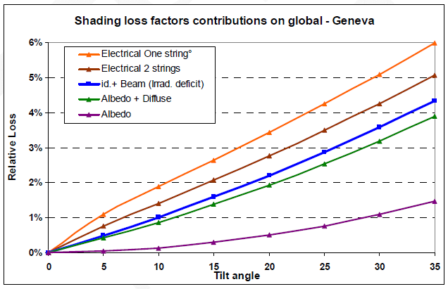
Even with backtracking strategy, the simulation shows a shading loss due to the diffuse (and albedo), which is usually between 2 and 3%. See the other post How is calculated the shading loss on diffuse with tracking systems ? People sometimes compare this loss to the loss of row-like (sheds) systems with fixed orientation, which may be much lower, depending on the system. How to explain this ? Please remember that with sheds systems, the shading loss strongly increases with the tilt of the sheds. Now with a tracker system, the tilt may obviously be very high in the morning or the evening, when the sun is low on the horizon. The picture shows the contribution of different irradiance losses in a shed system, as function of the tilt, for a given "limit angle" of 20° (i.e. pitch increasing when the tilt increases). Shading loss contributions as a function of tilt First, we observe that the Albedo contribution is important. The transposition model involves an albedo contribution proportional to (1 - cos(tilt))/2, i.e. low at usual tilts (e.g. 4.7% for tilt=25°), but significant at high tilts (25% at 60°). Then, as only the first tracker "sees" the albedo of the ground in front of the system, the albedo is affected by a shading factor of (n-1)/n, where n = number of sheds. This means that the albedo contribution is almost completely lost in big systems Secondly, the loss on the diffuse (sky masked by the preceding shed) is also significant, and strongly increasing with the tilt. The diffuse shading factor is the result of an integral over the sky vault, of the shaded parts multiplied by the cosine of the incidence angle of each "ray". Therefore a hiding band of the preceding tracker has a much higher effect when the plane (tracker) is at high tilt of 60°, as the cosine of the incidence angle of the bottom of the next shed is higher (cos 30°=0.866). If your plane is 15° tilt (sheds configuration), the plane will "see" the next shed with an incidence angle of the "shaded" rays of the order of 75°, i.e. a cos(75°) = 0.25. With backtracking strategy, the evolution of this shading loss is not varying much as function of the pitch, even for very large pitches. This is explained by the fact that with narrow pitches, the backtracking amplitude is low, when with large pitches, the trackers may take much higher tilts. And also because the loss of the albedo component is the same whatever the pitch between trackers for a given tilt (the albedo is masked as soon as the profile angle is higher than 0°).

-
In this case you can take the efficiency of the inverter at PNom (i.e. the extremity of the efficiency curve). By the way this value is not critical in the approximate evaluation described in the Help. We are aware that this definition is not quite satisfactory, and we are preparing a new approach using the effective transformer properties.