
Luca Antognini
-
Posts
14 -
Joined
-
Last visited
Everything posted by Luca Antognini
-
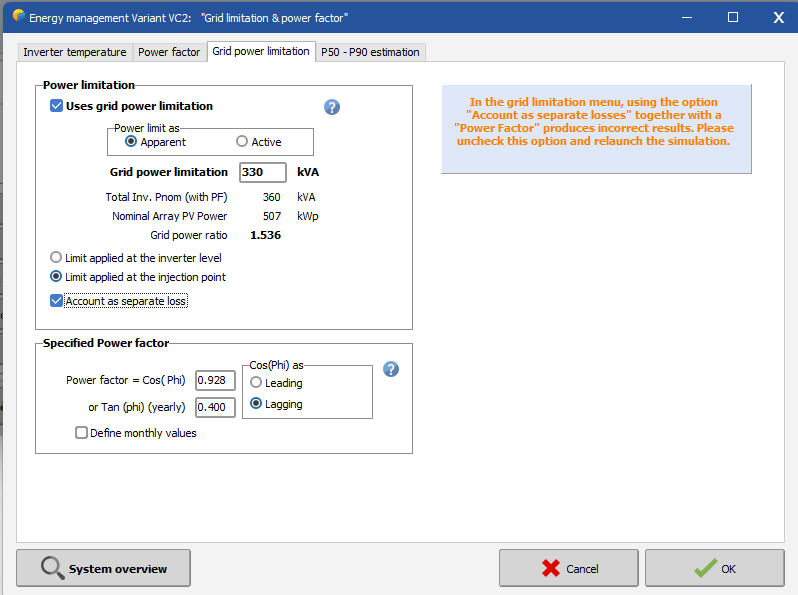
 Grid Power Limitation: The option "Account as separate loss" in the menu grid power limitation poses a problem when used together with a power factor. Indeed, at the moment, the reactive energy produced is computed based on the available energy at the output of the inverter. When a grid limitation is present, this is acting normally as a clipping loss on the inverter, therefore the available energy at the output of the inverter is reduced and so is the reactive energy. However, when the option "account as separate loss" is used, the energy at the output of the inverter is virtually higher, causing a miscalculation of the reactive energy. It depends on the magnitude of the grid limitation, so we recommend users to check their simulation with and without this option to decide whether or not to use it. Until the option is fixed in a future version, the software will display a warning when both options are used together.
-
Arev factor of BC modules in string level simulation
Luca Antognini replied to Chen's topic in Problems / Bugs
Dear Jianguo Chen, Thank you for your feedback. I share your understanding : both dialogues, with those parameters, should lead to the same results. For me the correct plot is your top screenshot, from the menu "One shaded Module". I noted that this problem seems to happen only with "Twin-half-Cut" module: If I select a "In length" module, both dialoguess give me the same results I think therefore there is a problem with the calculation of the electrical layout in this specific dialog. I will create an issue to investigate it further and fix this problem in a future version. -
You can find the detailed explanation to your question in our documentation on the power factor : https://www.pvsyst.com/help/project-design/grid-connected-system-definition/power-factor/index.html Check in particular: https://www.pvsyst.com/help/project-design/grid-connected-system-definition/power-factor/Simulation results.html In short: the power factor that you set in the menu "Energy management", here cos(phi)=0.9, is the power factor at the inverter level. The reactive power will be computed from the available power at the output of the inverter as EReGrid=EOutInv×tan(ϕ). We assume that there is no loss of reactive energy from the inverter to the injection point. However, we assume active energy loss in the AC circuit. Therefore, the power factor at the injection point will be decreased compared to the setting at the inverter output.
-
Hello, By definition a .PAN represents a PV modules with its performance. Even withing the same technology, there are a lot of variations of solar cell performance - from providers, from batch-to-batch, from improvement in the production line etc... So if you change the solar cells, it becomes a completly different product and all the values entered in the .PAN file should be reviewed for consistency. Now it all depends what is your simulation goal by doing this. I can only answer your question if you give me more details and context.
-
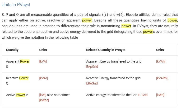
Hi! Yes E_Grid is an "active" energy/power. You can find explanation about active, reactive and apparent energy on the page: https://www.pvsyst.com/help/project-design/grid-connected-system-definition/power-factor/index.html?h=power+facto#apparent-reactive-and-active-power-definition The table at the end of the page give you the different definitions: Upon defining a power factor through the menu "Energy Management / Power Factor", the two additional variables EReGrid and EApGrid become available in the detailed results and also appear in the loss diagram.
-
How to simulate Tandem data of top and bottom cells
Luca Antognini replied to Shurouq's topic in How-to
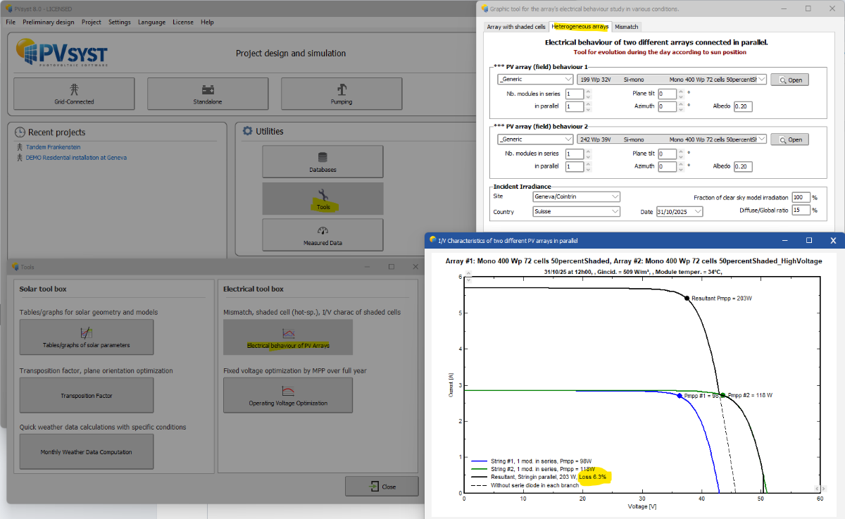
Hello, We are starting to think about the question of simulating TANDEM solar cells in PVsyst, but unfortunately for the moment it is not possible. The behaviour of the two absorbers with temperature and solar spectrum is not trivial and we need to implement a few models to describe it. Though, I believe the case of 4T (both cells connected in parallel) can be more easily approximated than the 2T case (both cells connected in series), as voltage mismatches create usually less power losses than current mismatches. I will give here an attempt to set up PVsyst to approximate a 4T Tandem behaviour in the present version of the software (8.0). But bearin mind that this is a very preliminary approach and require more testing. 1) Create two .Pan files, one to represent the top cell, one to represent the bottom cell, as if they were measured independently. This way you set up the one diode parameters for each cell. Use the same number of cells, modules dimensions etc... 2) Create a system with two subarrays, one with each .Pan files, with same number of panels connected in series and number of strings in both. Connect them to a same inverter and use the power sharing feature. You will not be able to connect the two subarrays to a single MPPT here, so at this stage we are neglecting the voltage mismatch (see next step). 3) Advanced losses / Module Quality LID Mismatch / Strings Voltage Mismatch: You can add here a general percentage to represent the loss of power due to the mismatch. To evaluate this one, you can use PVsyst specific tools > Electrical Behaviour of PV Array > Heterogeneous array. Here you can select your two .PAN files and open the I/V graphs. It will show you the percentage loss due to the mismatch between both modules for a given time of the day and date. Vary a bit those one and you will notice that this percentage is almost constant, as voltage mismatch should behave. Report this number in the Advanced losses. 4) Thermal model: We also need to tweak PVsyst regular parameters. With our setup, PVsyst will see two independent panels with low efficiency (~<15%), and therefore calculate that they are dissipating a lot of energy into heat. Which is not correct since in reality we have a single device with high efficiency (>30%), so more electricity, less heat. We need therefore to adapt the coefficients of the thermal model (https://www.pvsyst.com/help/project-design/array-and-system-losses/array-thermal-losses/index.html#thermal-model) According to the equation of the thermal model Tcell=Tamb+(Alpha⋅Ginc⋅(1−Effic))/U we could correct the model by using a different U value to compensate for the wrong (1-Effic) term. In my example (assuming single cells efficiency at ~15% and Tandem at about ~30%), the corrected value would become U_corr = U * (1-0.15) / (1-0.3) = U * 1.21. So in the case of open rack, instead of using the values of Uc = 29 W/m2/K, use something slightly larger Uc_corr = 35 W/m2/K. This will lower the losses of 1-2%. 5) Spectral correction: Unfortunately, I haven't reflected yet on how to adapt the spectral correction for the Tandem case. I think this cannot be guessed and of course the behaviour will be different than crystalline silicon. But you should keep in mind that it might be an import factor that we ignored too here! Please do not hesitate to comment on the approach. And as said above, we are reflecting on what model to implement in the future for dealing with 2T and 4T tandem devices, so any input would be useful for us : )
-
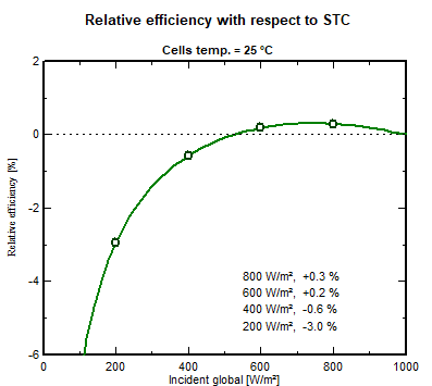
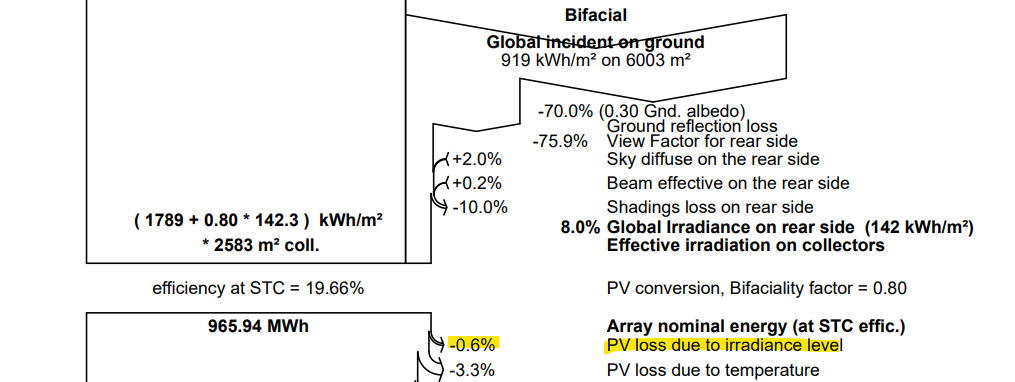
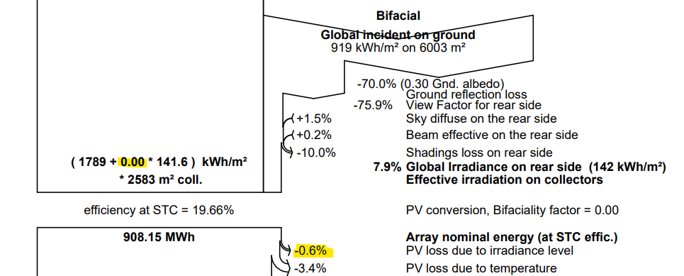
Careful, the 200W/m2 I indicated was not refering to the rear side irradiance. It was a lower irradiance level, irrespective of whether the front or the rear recieves it. I would agree with your calculation only in the case where the front side doesn't recieves any light. Otherwise you cannot decompose the efficiency in two parts from front and rear, it doesn't add up linearly. You need to consider the full I-V curve under the effective irradiance of both front and read sides together. ----- Let's take other numbers to not create confusion again. If in certain scenario, the front side recieves 1000 W/m2 and the rear side e.g. 50W/m2, the module recieves an equivalent of 1000 + f*50 W/m2 of total irradiance. Let's say f=0.8, it is 1040W/m2. If the irradiance level is lower, let's say 5 times lower, the front side recieves 200 W/m2 and the rear side 10 W/m2. Thereforer, under low light, the module recieves an equivalent of 208 W/m2 in total. The curve of performance of the module as function of irradiance should be understood as function of this effective total irradiance. (Indeed, in the norms, when bifacial module are measured, the rear side is masked to not absorbed any light from the rear.) You can visualize this curve in the .PAN file: So whether the light comes from the rear or the front, it is the Incident global light that matters. For this specific curve, if the Incident global Incident global = front-side irradiance + (rear-side irradiance × bifaciality factor) is equal to 200 W/m2, the efficiency will be -3.0% lower than if the Incident global was 1000 W/m2. So any module PV module, bifacial or not, under given illumination condition will operate somewhere on this curve. If the module operates above the reference of 1000 W/m2, you have an efficiency degradation with respect to STC, between 500-1000 W/m2 (for this particular example), you have an efficiency boost, below 500 W/m2 you have an efficiency degradation. It doesn't matter if it is bifacial or not. However, the bifaciality has this influence that the module will operate at a higher illumination level than a monofacial counterpart (in the hypothesis they have exactly the same electrical properties), so at another position on this curve. But as you can see, it could well either mean an improved performance! PVsyst of course take this into account during simulation and you can find it in the loss diagram. For example if you use the "Demo Commercial Oakland" with VC6, you can see it there If for the sake of the test, you modify the .PAN file and set the bificiality factor to 0, you get then: Therefore, for this specific example, on the yearly production you don't see a specific loss difference due to the irradiance level operating further from STC between a bifacial and monofacial module. This is because this effect is small here (I would call it a third order correction). If you had a system with better Albedo for example, the comparison could be different.
-
Clarifying Definitions to Avoid Confusion At PVsyst, the term "low-light performance" is usualy defined in the context of a PV module illuminated solely from the front side. Let’s consider the following example: At a reference irradiance of 1000 W/m², the module has an efficiency of 22% At a lower irradiance of 200 W/m², the efficiency drops slightly to 21.34% We define low-light performance as the relative difference in efficiency: (21.34 - 22) / 22 × 100 = -3% (relative) This means the efficiency at the lower light level is 3% lower relative to that at full irradiance. This is the standard definition used in PVsyst. Important Note: A more negative number (e.g., -4%rel or -5%rel) does not necessarily imply worse performance. In fact, it often indicates that the module performs better at high irradiance (1000 W/m²), which is an observed trend in modern PV modules, largely due to reduced series resistance Bifacial Modules and Rear-Side Illumination When it comes to bifacial modules, if only the rear side is illuminated (for the sake of the discussion), the module’s efficiency is proportional to the front-side efficiency, scaled by the bifaciality factor f. This factor applies equally at both high and low light levels. Therefore, the relative low-light performance of the rear side is identical: (f × 21.34 - f × 22) / (f × 22) = -3% (relative) Link to the Bifaciality Factor Definition To relate this to my colleague’s earlier explanation: the bifaciality factor is defined as the ratio of power output when the module is illuminated from the rear versus the front. This difference in power is primarily due to optical property differences between the two sides of the solar cell. Indeed: The cell materials are different on the front and rear sides Any differences in charge transport or extraction are negligible (These effects are much much smaller than the typical uncertainty in datasheet bifaciality (e.g., 80% ± 5%)) Thus, the bifaciality factor can effectively be understood as a scaling factor for the photogenerated current. In practical terms, the total irradiance received by a bifacial module can be calculated as: Irrad_Tot = front-side irradiance + (rear-side irradiance × bifaciality factor) The PV module performance modeling can then proceed without needing to differentiate which side the light is coming from—the model is agnostic to the direction of light incidence and so is the low-light performance.
-
Modeling modules with different powers in a single MPPT
Luca Antognini replied to Gustavo Pianovski's topic in How-to
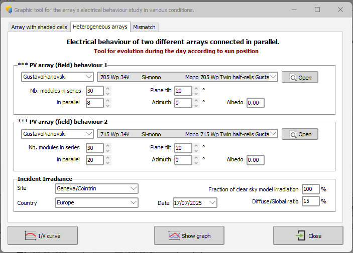
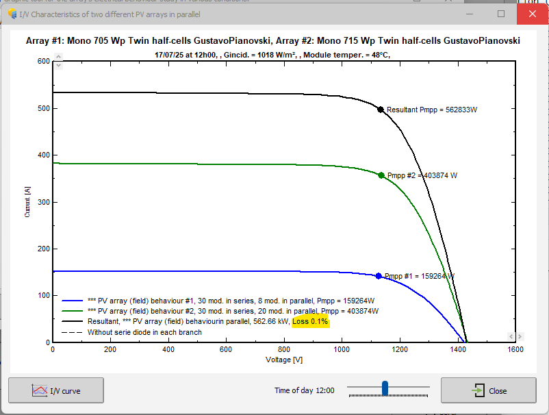
Hi! If you could provide the full detailed about the module (the missing Isc and voc values) that would be easier to reproduce your example. The simulation you want to describe consists of different strings connected in parallel into a single MPPT, which will create some small losses of voltage mismatch between the strings (they don't have all the same Vmpp). In this view, none of the two first simulations setup you describe can include this effet, as they both represent strings connected either to different MPPT or different inverters. They won't suffer from voltage mismatch and lead the same results as you pointed out. And there are no ways to define exactly the configuration you are describing from the system window (as this is quite an unusual one). The correct approach is indeed to add these losses later in the detailed losses menu, by evaluating them roughly (they are rather small in the end) independantly of the main simulation. Now, for the difference between your calculation and PVsyst calculation, I see first that in your table you update the voltages to lower values but keep the current unchanged. However, if you reduce the voltage from MPP, it will increase the current and therefore the power is slightly higher than in your evaluation. And consequently the losses would be smaller. It is really not surprising that PVsyst gives you such a small value when you have such as small difference of voltage among strings. Another impact you should consider is that the MPP of your configuration will be closer to the one of the strings formed of 710W and 715W pannels than the one of the string composed of the 705W, because they have much more strings in parallel (36 and 37 vs 8). Therefore there is more to loose to move the voltage for those one than for the 8 strings of 705W pannels. If you want to see this effect, you can also check it with another tool : Tools / Electrical behaviour of PV Arrays / heterogeneous arrays (note: the limit of the tool is 20 strings but it is not a problem for us). You can see that the relative losses are smaller than 0.1%. And this is already a pessimistic scenario here. So In the case of your system you could consider neglecting completly those voltage mismatch losses.
-
Dear Mikhail, The aging tool is a general tool to represent several situations. Unfortunately, the literature is a bit scarce on aging (real aging tests need years of field testing and there are a variations among technologies and climates - new technologies still need to be monitored more extensively) and on our side we don't have at the moment a clear literature review on the topic to hand out on to give clear recommendation on our side. However, here are a few additional clarifications: First recommendation: if provided, input the aver. degradation factor from the data sheet of your module (/!\ this is not equivalent to the warranty!). Know that average degradation factor lies between 0.2-0.6%/year. So you can adapt it if you want to see a more or less optimistic/conservator impact. The Imp / Vmp contribution is set by default to 80/20 %, to represent the fact that often the first impact on the long term are first of optical nature (=decrease the current), for example due to encapsulant yellowing. But this is to adapt with what you find in the literature about your technology or what you observe in the field. The Imp and Vmp RMS dispersion are tuning parameters of the model. If you set them at 0, all the PV modules will have the exact same degradation rate and your system will follow the blue curve. Set to higher values, the PV modules will have mismatch among them and an additional loss occurs because of this (mainly driven by the PV module whose current degrades the fastest). There is not really literature to advise what parameters to input here, but you can use this parameters to visualize the extra impact of this mismatch or tune it to make it correspond to existing measurements of a PV system.
-
Limitation of pan file for BC and HJT module
Luca Antognini replied to Chen's topic in Problems / Bugs
Dear Chen, We are currently investigating how to adapt our model to such technologies. It will take some times, as we want our modification to be backed-up by high quality experimental data and be applicable to the whole of our PV module database. We will present an update of our research at the upcoming EU-PVSEC. -
Hello, Thank you for reporting those behaviors. I believe there are several issues, which I will report for future correction, but my interpretation is different: - There are indeed a unit problem with the apparent and reactive energy, which will be corrected in future version. In the report, the switching to Mega watt hour instead of kilo watt hour doesn't work well for those quantity. The numerical value displayed is correct by the "k" in the unit doesn't switch yet to and "M". You can change the unit of the report for a consistent display in "kWh" by going to "Report > Report Options > Final Report Options > Energy Units > kWh". - The name of reactive and apparent energy are correctly displayed in the report. Though it seems to me that you didn't allow "solar injection into the grid" in the "self-consumption" window. Therefore, no active energy is transferred to the grid from the solar production and reactive and apparent energy are equal: Note here that the reactive component is computed based on the solar energy available at the inverter's output, as E_Reac = E_InvOut * Tan(phi). Then the apparent energy is E_app = sqrt (E_Reac*E_Reac + E_Act*E_Act) Let me know if this makes sense for you. As I see that you are trying to simulate a scenario with a large consumption, you were maybe looking for a different behavior of the reactive energy. Luca
-
Units of Energy in PVsyst 8760 CSV Output File
Luca Antognini replied to kjs55's topic in Suggestions
Hi! The variable in the hourly energy variables are sometimes displayed with units "kW" instead of "kWh". This is indeed a bit confusing but for time step of one hour this is equivalent. The case of the apparent and reactive energy units should be unified with the rest in the future. In particular the reactive energy should be displayed by convention in kVARh instead of kVAh (even though they are all pseudo-units, equivalent to kW in the end).