Luca Antognini

Hello, In the simulation, the Arev factor and reverse characteristic is not influenced by temperature nor irradiance level. Is that what you're asking? Please consult also our Q&A on how to simulate those device in PVsyst in the current version:

No specialized implementation yet, but you can consult our recent Q&A on the topic to understand the impact of BC cell and what workaround can be put in place to simulate them in PVSyst:

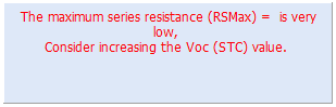
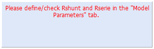
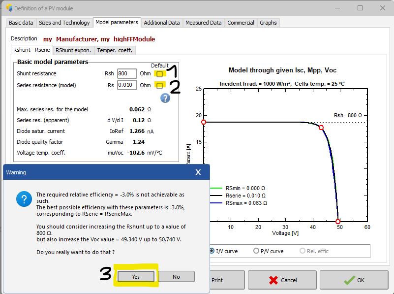
We research the topic (see our abstrac from EUPVSEC) but no new implementation at this stage. For the moment we still propose the following workaround: Problem for one diode model parameter determination with High fill factor PV modules: When entering a PV module in the database with a very high Fill Factor (above ~ 82-83%), or equivalently very high Vmp/Voc (above ~86%), PVsyst might not be able to find suitable parameters for the one diode problem and the following messages might appear: or This comes from the fact that PVsyst needs to find parameters that simultaneously reproduce several constraints and there might not exist a mathematical solution. This is a known mathematical problem, and more information is available in our dedicated publication : https://www.pvsyst.com/en/company/publications/ The solution we propose at the moment is to increase slightly Voc until PVsyst is able to find a solution. Note well that this does not impact the MPP, therefore the simulation results remain mostly unchanged by this small work around. PVsyst will find the minimum increase of Voc required if you do the following: 1) Go in the Tab "Model Parameters" 2) Check the box to get the default value of Rshunt: A pop-up will appear informing you of the impact on the relative low-light efficiency. Click Yes to close it. 3) Check the box to get the default value of Series resistance. Another pop-ip will appear informing you that in order to find a series resistance suitable with a relative low-light efficiency of -3% (the default value we suggest), PVsyst will need to increase the shunt resistance and possible the Voc value. Again click Yes to accept

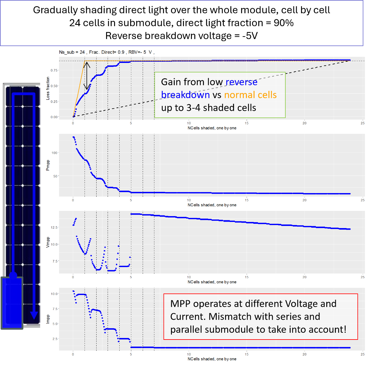
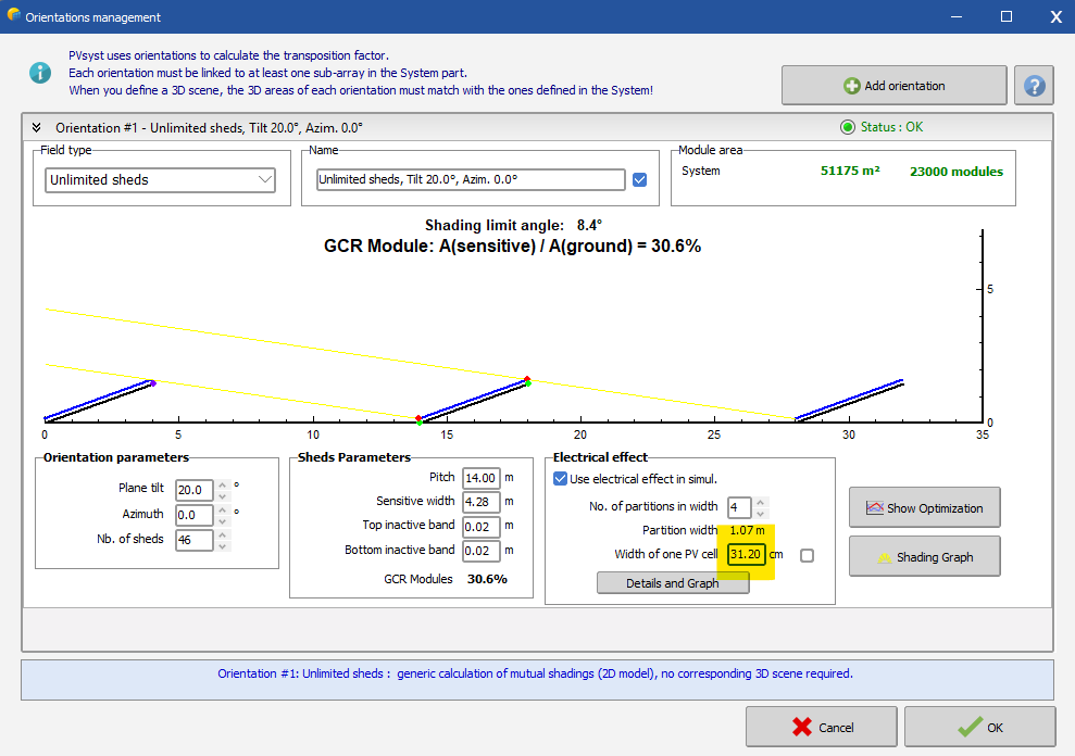
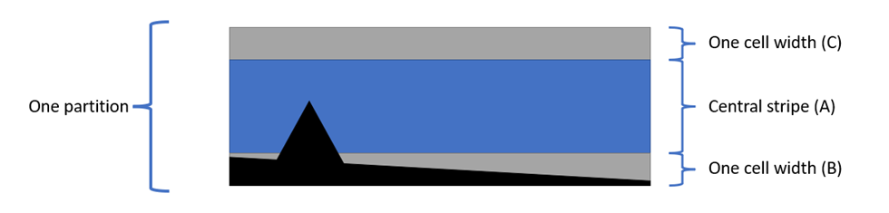
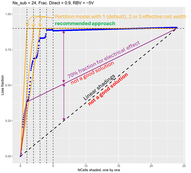
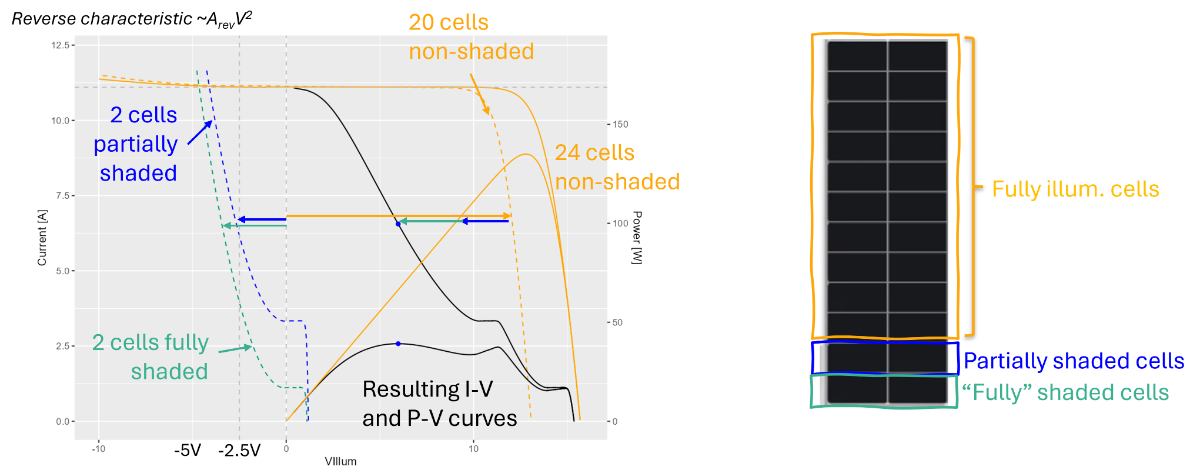
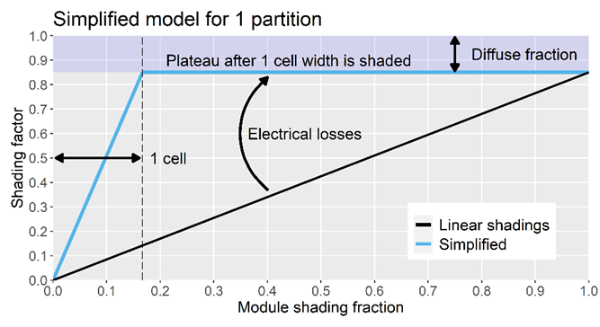
Summary: - Low reverse breakdown solar cells have a stronger shading tolerance than conventional modules in situations where less than 3-4 cells are shaded. - In the case of mutual shading of large systems with a row arrangement, we recommend to approximate their behaviour in PVsyst using the shading model of the "Unlimited sheds" or "Unlimited Trackers" orientation, using as input a cell width 2-3 times larger than the real value. - In the very specific case where shading on 3-4 cells or fewer occurs very often we have no precise recommendations. But since those situations occur rarely in large row-based systems, we recommend to stick to the usual recommendations of usage of the partition and module layout model. Since shading situations with 3-4 shaded cells happen rarely in large system, we estimate that neglecting this effect will not lead to significant errors in the yearly yield calculation. Therefore, PVsyst currently handles PV modules with IBC cells in the same way as other crystalline Si modules. Nevertheless, we intend to include the special behavior of IBC cells into our models, in order to account for this small improvement. The current roadmap foresees the availability of this feature by end of this year. In the meantime, the above described workaround should allow to approximate the results in a satisfying way. Q&A index: 1) What are the common misconceptions when using PVsyst to simulate low reverse breakdown voltage (RBV) solar cells? 2) How does the shading tolerance of PV modules featuring low RBV cells physically work? 3) How to simulate low RBV cells in PVsyst using the "Unlimited sheds" or "Unlimited trackers" case? 4) How to simulate low RBV cells for other shading scenarios? 5) What are the limitations of PVsyst shading models for 3D scenes when simulating low RBV cells and what are the recommendations? 6) Why modifying the electrical shading factor is not recommended to simulate low RBV cells? 7) Why modifying the Arev factor in the .PAN file does not improve representation of low RBV cells? - - - - - - - - - - - - - - - - - - - - - - - - - - - - - - - - - - - - - - - - - - - - - - - - - - - - - - - - - - - - - - - - - - - - - - - - - - - - - - - - - - - - - - - - 1) What are the common misconceptions when using PVsyst to simulate low reverse breakdown voltage (RBV) solar cells? We noted a few points of misunderstanding in the way the community tries to run PVsyst simulations for low reverse breakdown voltage (RBV) solar cells, such as some back-contact cells technologies. This answer aims at correcting those views, stating clearly what can or cannot be simulated in PVsyst at the moment, and how. Some common incorrect beliefs around this topic are: /!\ That each cell acts as its own bypass diode and therefore shading a cell doesn't lead to additional electrical shading losses. /!\ That, following the previous belief, the partition model can approximate the behaviour of those cells by setting a large number of partitions: This, however, strongly underestimates the voltage and current mismatch between the submodules. /!\ That it is possible to adjust the electrical shading fraction to fit those cells' behaviour: As we will see, this is in reality a poor fit to the real behaviour. /!\ That the module layout model is accurate for any arbitrary shading scenario: It is actually agnostic to the number of shaded cells, which matters for the precise description of low RBV cells. These misconceptions are related both to the understanding of the physics of the low RBV cells as well as to the understanding of the limitations of PVsyst shading models. Therefore we shall cover both topics: 2) How does the shading tolerance of PV modules featuring low RBV cells physically work? Low RBV cells have the advantage of allowing significant current to flow already at moderate reverse voltages. According to the literature, those cells allow a current around ~10 A at a reverse voltage of around -5.0 V to -2.5 V. This is indeed analogous to the working principle of a bypass diode in parallel with a string of cells (submodule), except it would be as if each cell possessed its own bypass diode. However, as in the case of a regular bypass diode, the reverse operation of a low RBV cell leads to a voltage loss. For example, in a string of 24 low RBV cells under illumination, a fully shaded cell will operate at around -5 V, reducing the total voltage of the string. Increasing the number of shaded cells drastically reduces the voltage of the string: Number of shaded cells Number of remaining illuminated cells String voltage 0 24 14.4 ( ~0.6 x 24) 1 23 8.8 2 22 3.2 3 21 string operates in reverse => bypass diode activation This simple estimation shows us immediately that the benefit of the low RBV technology is only present in shading scenarios where only a few cells (3-4) are shaded, due to the significantvoltage loss created by those cells. In shading situations where more cells are shaded, low RBV cells perform the same way as regular cells due to the bypass diode activation. To be more rigorous, we show in the following figure a more precise computation resulting from the summation of the I-V curves of each cell of a submodule of 24 cells. For this example, the direct light is fully shaded for one cell and partially shaded for another, while the remaining cells are fully illuminated. This shows how voltage is loss in the shaded cells and how the MPP can abruptly shift to lower voltages. The next figure is created using the same method, gradually varying the number of shaded cells: Compared to a regular cell (in orange), which features a sharp rise in losses after a single cell is shaded, the low RBV technology mitigates these losses when less than 3-4 cells are shaded (as expected from the simple estimation). Above this, the only power remaining comes from the unshaded diffuse light, as for regular cells. Moreover, we note that the operating point (Impp, Vmpp) follows a distinctive pattern for this technology. If this submodule is connected in series (parallel) with unshaded submodules operating at another current (voltage), the benefit of the low RBV technology will be lost because an electrical mismatch loss will occur. An example is the common case of twin half-cell modules, where the top supbmodule is connected in parallel to the bottom one: In a shading scenario where a shadow comes from the lower part of the submodule, the voltage mismatch created between the top and bottom submodules mitigates completly the benefit of the low RBV technology! 3) How to simulate low RBV cells in PVsyst using the "Unlimited sheds" or "Unlimited trackers" case? As described above, the benefit of low RBV cells is only present in very specific shading scenarios AND electrical connections. The latest version of PVsyst (8.0 and the upcoming 8.1) can approximate the behaviour of low RBV cells ONLY in very specific scenarios. Therefore, we can give recommendations only in the cases of "Unlimited sheds" or "Unlimited trackers", because in that case the shading scenario is very clear: the shadow comes gradually from the bottom of the modules. In that case: - For "in length" modules: double the effective cell size to get an upper bound on the production. - For "Twin half-cell" modules: the effect of the low reverse breakdown voltage is mitigated in this architecture. Use the usual recommendation for normal cell types. This can be easily tested in the Demo project "_DEMO_utiliy.PRJ". 4) How to simulate low RBV cells for other shading scenarios? For any other shading scenarios (inhomogeneous shading, thin objects, etc.), we can only recommend not treating the electrical shading with the linear model or with a high number of partitions: this would strongly underestimate the electrical shading losses. Sticking to the usual partition recommendation would be best, acknowledging that it might slightly overestimate the losses due to the cases where only 1 to 4 cells are shaded. 5) What are the limitations of PVsyst shading models for 3D scenes when simulating low RBV cells and what are the recommendations? PVsyst's shading models are unfortunately not adapted to simulate situations where the low RBV technology provides an advantage compared to other technologies, i.e. when only 3-4 cells per module are shaded. The reason is that PVsyst shading models are convient approximations for very large systems with regular shadows. More specifically, the limitations of each model regarding the representation of low RBV cells are: The linear shading model compute the losses proportionally to the shaded area, completely neglecting the electrical mismatch. The module layout method computes the I-V curves by summing them as a function of the number of shaded corners in each submodule. However, the I-V curves in this method are pre-calculated, and in the case where one corner of a submodule is shaded, it is not possible to determine whether 1, 2 or 3 cells are shaded (which would be important to represent the cases where low RBV cells outperform regular cells!). The partition model computes the losses according to the shading fractions of the three following stripes: If the central stripe is shaded, the loss factor is maximal. If only the top and/or bottom stripes are shaded, the loss is proportional to the shaded area up to a full cell area: This emulates very well the behaviour of low RBV cells in the case of a uniform shadow coming from the bottom of the module. But the model is agnostic about the shading fraction of each cell and cannot guarantee a good representation with irregular shading of the cells. In the future, we hope to be able to provide more detailed electrical shading loss calculations. 6) Why modifying the electrical shading factor is not recommended to simulate low RBV cells? Some users claim that the electrical shading factor could be used to approximate the benefit of low RBV cells. However, it does not match well with the results presented above, as it corresponds to the following attempt of fitting: /!\ Indeed, the electrical shading factor is meant for a very specific context within PVsyst: it is used to tune the partition model to match the simulation results of the module layout model. See this page. Instead, in the case of mutual shading in row-based large systems, we recommend to approximate their behaviour in PVsyst using the shading model of the "Unlimited sheds" or "Unlimited Trackers" orientation, using as input a cell width 2-3 times larger than the real value. 7) Why modifying the Arev factor in the .PAN file does not improve representation of low RBV cells? The Arev factor in the .PAN file is indeed meant to represent the reverse characteristic of solar cells. At the moment it is only taken into account within the module layout model. However, as explained above, the module layout does not have the sufficient resolution to differentiate situations where 1, 2 or 3 cells are shaded and therefore it does not represent well the behaviour of low RBV cells.

Hello James! ==> Beware that you are comparing those model on a single location: Erbs might could be less biased than DIRINDEX at another location. Usually, if those models were fitted on a dataset large enough, they should reach a very low global bias. ==> It always makes sense to improve our models, for hourly timescale as well. We compared so far the ability of Engerer2 and Erbs to reproduce ground measurement of 113 weather stations (IEA-PVPS dataset). We are going to carry this comparison more in depth for several additional model in the future, with in particular DIRINT, that is used for example by Meteonorm, and potentially DIRINDEX as well. These comparisons will serve the purpose of documenting our implementations of the models accross PVsyst version notably. However, those kind of study already exists in the literature, but none of them point to a universal model yet that would outperform greatly all the others. Edit: For the moment, for hourly simulation, the Erbs model is still used. Note well that those models are used only in the case of custom weather import where no DHI data are provided.

Hello, Sorry for this warning message, it is nothing to worry about. It doesn't impact the simulation and can be ignored. It will be removed in 8.1.01. It is related to the thermalisation time of your subarrays compared to the simulation timestep. But it should not have been classified as a warning, only an information for internal use at PVsyst - because it should be present in the back for conditions that are actually suitable for a good simulation.

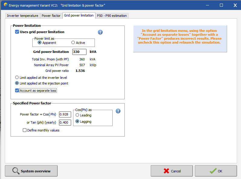
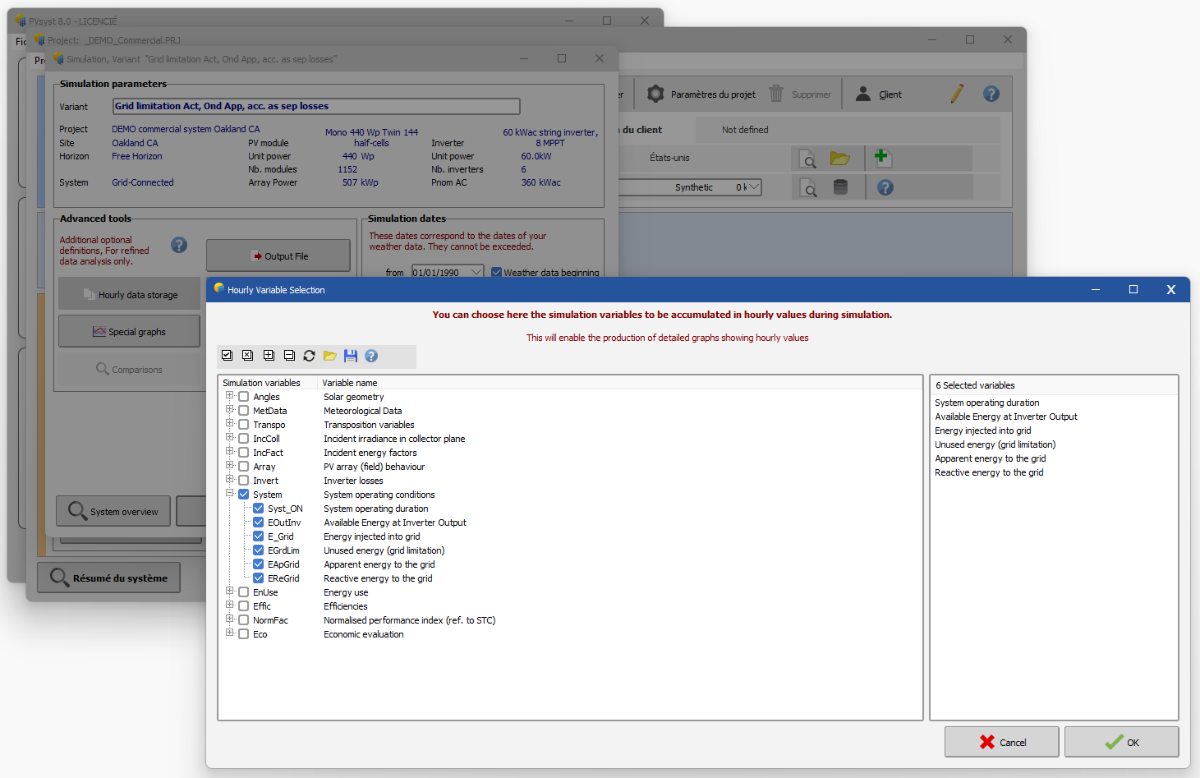
Grid Power Limitation: The option "Account as separate loss" in the menu grid power limitation may pose a problem when used together with a power factor. However the loss diagram and .csv simulation output are not affected. Hourly Graphs may be affected upon context: When the simulation variables EReGrid, EApGrid and EGrdLim are not explicitly saved, it can trigger wrong calculations of the reactive and apparent energy in the hourly plots (too high values for both). Saving those variables in the menu "Advanced simulation / Hourly data storage" solves the issue: Until the option is fixed in a future version, the software will display a warning when both options are used together.

Dear Jianguo Chen, Thank you for your feedback. I share your understanding : both dialogues, with those parameters, should lead to the same results. For me the correct plot is your top screenshot, from the menu "One shaded Module". I noted that this problem seems to happen only with "Twin-half-Cut" module: If I select a "In length" module, both dialoguess give me the same results I think therefore there is a problem with the calculation of the electrical layout in this specific dialog. I will create an issue to investigate it further and fix this problem in a future version.

You can find the detailed explanation to your question in our documentation on the power factor : https://www.pvsyst.com/help/project-design/grid-connected-system-definition/power-factor/index.html Check in particular: https://www.pvsyst.com/help/project-design/grid-connected-system-definition/power-factor/Simulation results.html In short: the power factor that you set in the menu "Energy management", here cos(phi)=0.9, is the power factor at the inverter level. The reactive power will be computed from the available power at the output of the inverter as EReGrid=EOutInv×tan(ϕ). We assume that there is no loss of reactive energy from the inverter to the injection point. However, we assume active energy loss in the AC circuit. Therefore, the power factor at the injection point will be decreased compared to the setting at the inverter output.

Hello, By definition a .PAN represents a PV modules with its performance. Even withing the same technology, there are a lot of variations of solar cell performance - from providers, from batch-to-batch, from improvement in the production line etc... So if you change the solar cells, it becomes a completly different product and all the values entered in the .PAN file should be reviewed for consistency. Now it all depends what is your simulation goal by doing this. I can only answer your question if you give me more details and context.

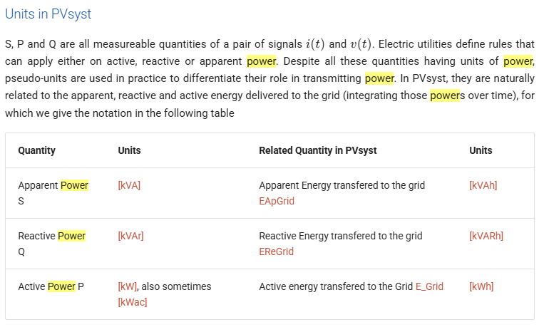
Hi! Yes E_Grid is an "active" energy/power. You can find explanation about active, reactive and apparent energy on the page: https://www.pvsyst.com/help/project-design/grid-connected-system-definition/power-factor/index.html?h=power+facto#apparent-reactive-and-active-power-definition The table at the end of the page give you the different definitions: Upon defining a power factor through the menu "Energy Management / Power Factor", the two additional variables EReGrid and EApGrid become available in the detailed results and also appear in the loss diagram.

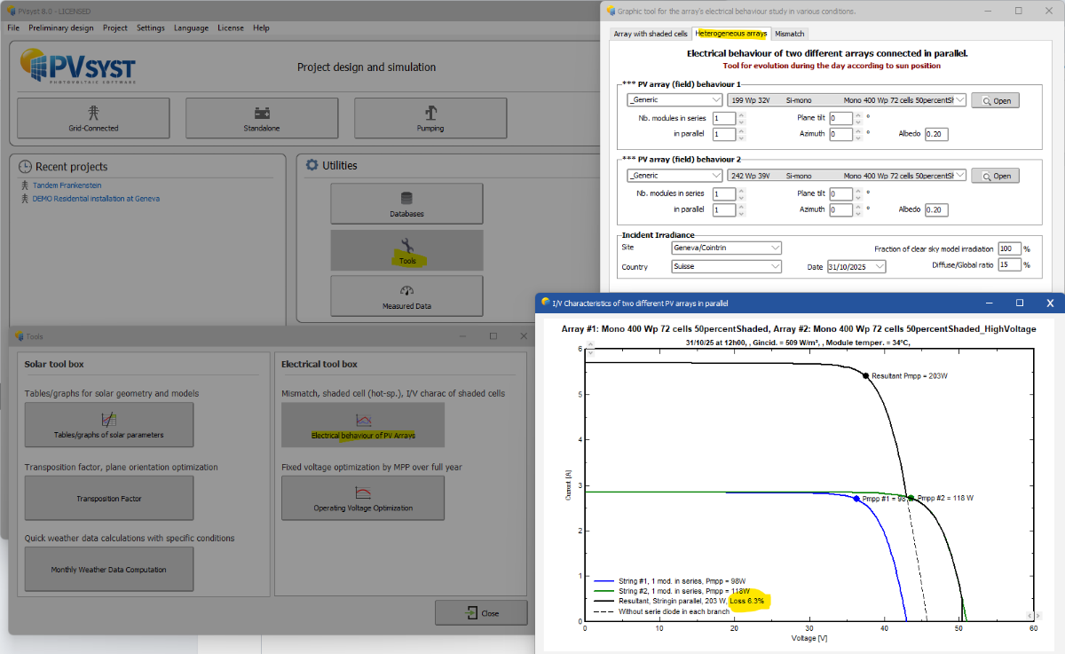
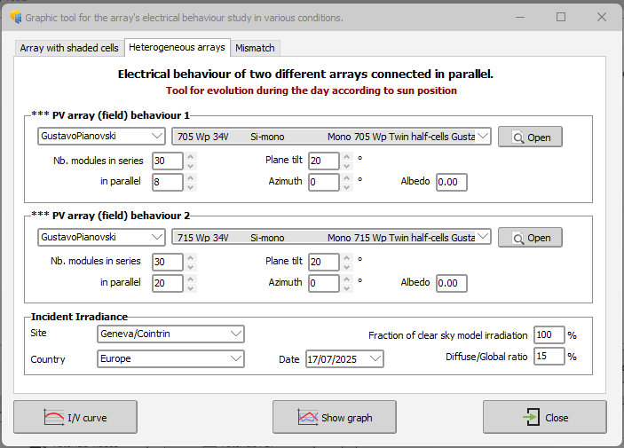
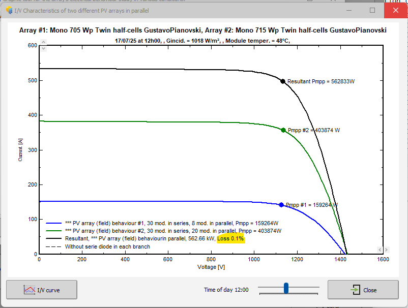
Hello, We are starting to think about the question of simulating TANDEM solar cells in PVsyst, but unfortunately for the moment it is not possible. The behaviour of the two absorbers with temperature and solar spectrum is not trivial and we need to implement a few models to describe it. Though, I believe the case of 4T (both cells connected in parallel) can be more easily approximated than the 2T case (both cells connected in series), as voltage mismatches create usually less power losses than current mismatches. I will give here an attempt to set up PVsyst to approximate a 4T Tandem behaviour in the present version of the software (8.0). But bearin mind that this is a very preliminary approach and require more testing. 1) Create two .Pan files, one to represent the top cell, one to represent the bottom cell, as if they were measured independently. This way you set up the one diode parameters for each cell. Use the same number of cells, modules dimensions etc... 2) Create a system with two subarrays, one with each .Pan files, with same number of panels connected in series and number of strings in both. Connect them to a same inverter and use the power sharing feature. You will not be able to connect the two subarrays to a single MPPT here, so at this stage we are neglecting the voltage mismatch (see next step). 3) Advanced losses / Module Quality LID Mismatch / Strings Voltage Mismatch: You can add here a general percentage to represent the loss of power due to the mismatch. To evaluate this one, you can use PVsyst specific tools > Electrical Behaviour of PV Array > Heterogeneous array. Here you can select your two .PAN files and open the I/V graphs. It will show you the percentage loss due to the mismatch between both modules for a given time of the day and date. Vary a bit those one and you will notice that this percentage is almost constant, as voltage mismatch should behave. Report this number in the Advanced losses. 4) Thermal model: We also need to tweak PVsyst regular parameters. With our setup, PVsyst will see two independent panels with low efficiency (~<15%), and therefore calculate that they are dissipating a lot of energy into heat. Which is not correct since in reality we have a single device with high efficiency (>30%), so more electricity, less heat. We need therefore to adapt the coefficients of the thermal model (https://www.pvsyst.com/help/project-design/array-and-system-losses/array-thermal-losses/index.html#thermal-model) According to the equation of the thermal model Tcell=Tamb+(Alpha⋅Ginc⋅(1−Effic))/U we could correct the model by using a different U value to compensate for the wrong (1-Effic) term. In my example (assuming single cells efficiency at ~15% and Tandem at about ~30%), the corrected value would become U_corr = U * (1-0.15) / (1-0.3) = U * 1.21. So in the case of open rack, instead of using the values of Uc = 29 W/m2/K, use something slightly larger Uc_corr = 35 W/m2/K. This will lower the losses of 1-2%. 5) Spectral correction: Unfortunately, I haven't reflected yet on how to adapt the spectral correction for the Tandem case. I think this cannot be guessed and of course the behaviour will be different than crystalline silicon. But you should keep in mind that it might be an import factor that we ignored too here! Please do not hesitate to comment on the approach. And as said above, we are reflecting on what model to implement in the future for dealing with 2T and 4T tandem devices, so any input would be useful for us : )

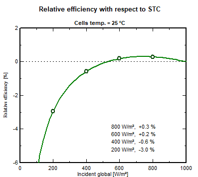
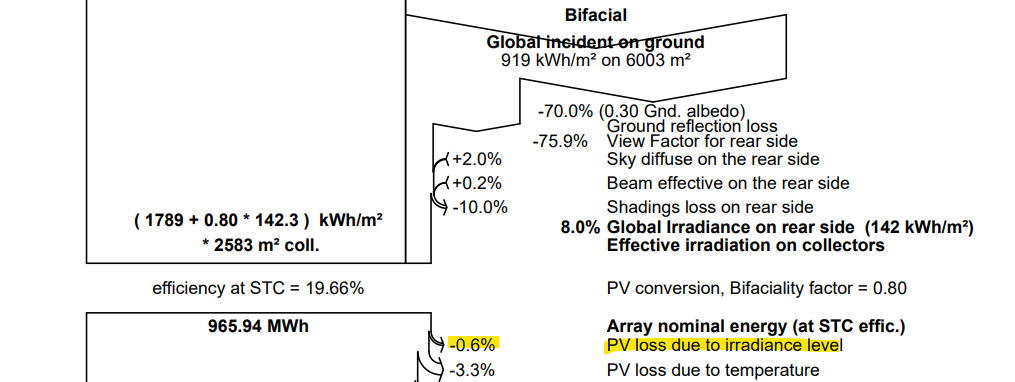
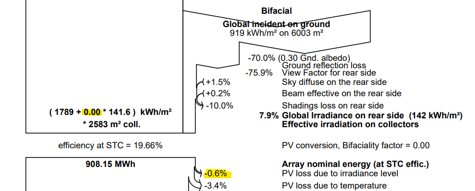
Careful, the 200W/m2 I indicated was not refering to the rear side irradiance. It was a lower irradiance level, irrespective of whether the front or the rear recieves it. I would agree with your calculation only in the case where the front side doesn't recieves any light. Otherwise you cannot decompose the efficiency in two parts from front and rear, it doesn't add up linearly. You need to consider the full I-V curve under the effective irradiance of both front and read sides together. ----- Let's take other numbers to not create confusion again. If in certain scenario, the front side recieves 1000 W/m2 and the rear side e.g. 50W/m2, the module recieves an equivalent of 1000 + f*50 W/m2 of total irradiance. Let's say f=0.8, it is 1040W/m2. If the irradiance level is lower, let's say 5 times lower, the front side recieves 200 W/m2 and the rear side 10 W/m2. Thereforer, under low light, the module recieves an equivalent of 208 W/m2 in total. The curve of performance of the module as function of irradiance should be understood as function of this effective total irradiance. (Indeed, in the norms, when bifacial module are measured, the rear side is masked to not absorbed any light from the rear.) You can visualize this curve in the .PAN file: So whether the light comes from the rear or the front, it is the Incident global light that matters. For this specific curve, if the Incident global Incident global = front-side irradiance + (rear-side irradiance × bifaciality factor) is equal to 200 W/m2, the efficiency will be -3.0% lower than if the Incident global was 1000 W/m2. So any module PV module, bifacial or not, under given illumination condition will operate somewhere on this curve. If the module operates above the reference of 1000 W/m2, you have an efficiency degradation with respect to STC, between 500-1000 W/m2 (for this particular example), you have an efficiency boost, below 500 W/m2 you have an efficiency degradation. It doesn't matter if it is bifacial or not. However, the bifaciality has this influence that the module will operate at a higher illumination level than a monofacial counterpart (in the hypothesis they have exactly the same electrical properties), so at another position on this curve. But as you can see, it could well either mean an improved performance! PVsyst of course take this into account during simulation and you can find it in the loss diagram. For example if you use the "Demo Commercial Oakland" with VC6, you can see it there If for the sake of the test, you modify the .PAN file and set the bificiality factor to 0, you get then: Therefore, for this specific example, on the yearly production you don't see a specific loss difference due to the irradiance level operating further from STC between a bifacial and monofacial module. This is because this effect is small here (I would call it a third order correction). If you had a system with better Albedo for example, the comparison could be different.

Clarifying Definitions to Avoid Confusion At PVsyst, the term "low-light performance" is usualy defined in the context of a PV module illuminated solely from the front side. Let’s consider the following example: At a reference irradiance of 1000 W/m², the module has an efficiency of 22% At a lower irradiance of 200 W/m², the efficiency drops slightly to 21.34% We define low-light performance as the relative difference in efficiency: (21.34 - 22) / 22 × 100 = -3% (relative) This means the efficiency at the lower light level is 3% lower relative to that at full irradiance. This is the standard definition used in PVsyst. Important Note: A more negative number (e.g., -4%rel or -5%rel) does not necessarily imply worse performance. In fact, it often indicates that the module performs better at high irradiance (1000 W/m²), which is an observed trend in modern PV modules, largely due to reduced series resistance Bifacial Modules and Rear-Side Illumination When it comes to bifacial modules, if only the rear side is illuminated (for the sake of the discussion), the module’s efficiency is proportional to the front-side efficiency, scaled by the bifaciality factor f. This factor applies equally at both high and low light levels. Therefore, the relative low-light performance of the rear side is identical: (f × 21.34 - f × 22) / (f × 22) = -3% (relative) Link to the Bifaciality Factor Definition To relate this to my colleague’s earlier explanation: the bifaciality factor is defined as the ratio of power output when the module is illuminated from the rear versus the front. This difference in power is primarily due to optical property differences between the two sides of the solar cell. Indeed: The cell materials are different on the front and rear sides Any differences in charge transport or extraction are negligible (These effects are much much smaller than the typical uncertainty in datasheet bifaciality (e.g., 80% ± 5%)) Thus, the bifaciality factor can effectively be understood as a scaling factor for the photogenerated current. In practical terms, the total irradiance received by a bifacial module can be calculated as: Irrad_Tot = front-side irradiance + (rear-side irradiance × bifaciality factor) The PV module performance modeling can then proceed without needing to differentiate which side the light is coming from—the model is agnostic to the direction of light incidence and so is the low-light performance.

Hi! If you could provide the full detailed about the module (the missing Isc and voc values) that would be easier to reproduce your example. The simulation you want to describe consists of different strings connected in parallel into a single MPPT, which will create some small losses of voltage mismatch between the strings (they don't have all the same Vmpp). In this view, none of the two first simulations setup you describe can include this effet, as they both represent strings connected either to different MPPT or different inverters. They won't suffer from voltage mismatch and lead the same results as you pointed out. And there are no ways to define exactly the configuration you are describing from the system window (as this is quite an unusual one). The correct approach is indeed to add these losses later in the detailed losses menu, by evaluating them roughly (they are rather small in the end) independantly of the main simulation. Now, for the difference between your calculation and PVsyst calculation, I see first that in your table you update the voltages to lower values but keep the current unchanged. However, if you reduce the voltage from MPP, it will increase the current and therefore the power is slightly higher than in your evaluation. And consequently the losses would be smaller. It is really not surprising that PVsyst gives you such a small value when you have such as small difference of voltage among strings. Another impact you should consider is that the MPP of your configuration will be closer to the one of the strings formed of 710W and 715W pannels than the one of the string composed of the 705W, because they have much more strings in parallel (36 and 37 vs 8). Therefore there is more to loose to move the voltage for those one than for the 8 strings of 705W pannels. If you want to see this effect, you can also check it with another tool : Tools / Electrical behaviour of PV Arrays / heterogeneous arrays (note: the limit of the tool is 20 strings but it is not a problem for us). You can see that the relative losses are smaller than 0.1%. And this is already a pessimistic scenario here. So In the case of your system you could consider neglecting completly those voltage mismatch losses.