

Vinh Thinh
-
Posts
10 -
Joined
-
Last visited
-
Dear all, I am reaching out whoever can help me with this topic. For several projects for which I am assessing the meteo data, there has been a potential misalignment between the on-site plane of array irradiation data registered by sensors (such as pyranometers or solarimeters) and Solargis satellite data. For this reason, I am questioning whether such occurrence has ever been encountered by someone else and if so, what has been the take-away. I am open to discussion on this topic. Thank you and best regards, Vinh
-
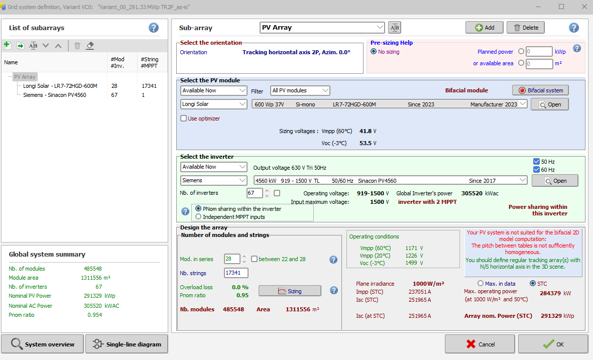
Hi, thanks for the answer. My problem is that when I import the pvc file with the shading scene I do not know how to associate the different pitch to the two system sub-arrays. Like in this case, I have already created two sub-arrays in System design for the two pitch values, but how can I associate them correctly? If I click on one of the two group of the 3D fields, it highlights a mix of trackers with the two different pitch values.

-
Hi Linda, how can I extract these data?
-
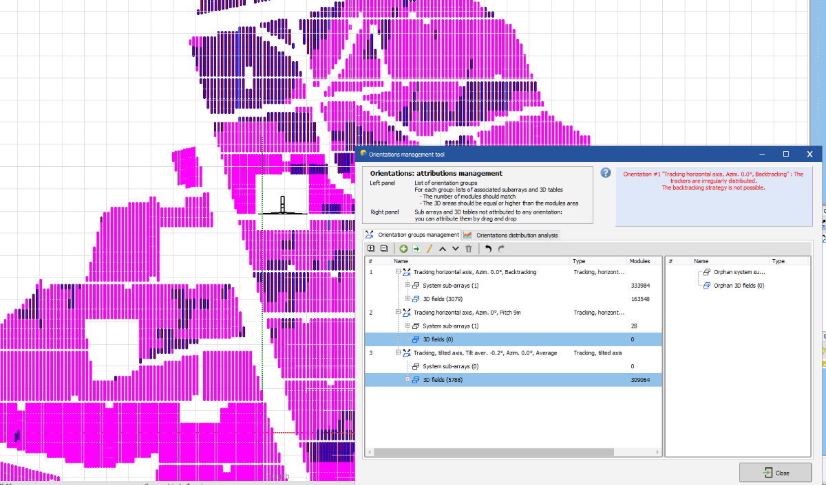
Hi All, I am currently using PVsyst version 8.0.9 and in the 3D scene, I am trying to export a .pvc file created with PVcase in which there are two different pitch values. While activating the bifacial features, I encounter an issue that does not allow to compute the simulation since the pitch is not sufficiently homogeneous. With PVsyst 8.0 is there a way to simulate in the same variant bifacial system with different pitch values? Am I trying to get the simulation in one single variant and not in two variants (one with a pitch of 9m and the other with pitch of 12m) and do the post-calculation. The reason is that I am trying to identify the impact of shadow casting of wind turbinesand those wind turbines are near trackers with both 9m pitch and 12 m pitch. Below, there is a screenshot of the problem. Any help is really appreciated. Best regards, Vinh
-
Hi again and thank you for your answer. I am still trying to figure out if there is a way to analyze the impact through the year of the shadow casting of the wind turbines. Like in my mind this are the steps I would follow: get the exported data on hourly basis for a year from the loss diagram, taking into account the %loss of near shading loss and electrical shading loss -> is it right? or should I take into account other losses for the shadings of the wind turbines? try to find a way to correlate the losses from the loss diagram through the year. Is there a study/methodology? For example, during Winter solstice I would have a bigger impact of shadows, so what fraction of the yearly near shading and electrical shading should I apply? and so through the year, on a monthly basis, how can I find the fraction of those year losses to be applied each month?
-
Thank you for the reply 🙂 Regarding your answer, I would like to have a better understanding on how to apply your procedure in order to visualize and quantify the shadowing impacts of turbines. First, I get that I shall generate two simulation variants one with and the other without them and from the two loss diagrams see the corresponding near shadings and electrical losses. In order to calculate those losses in MWh, if I understand correctly, I should multiply the energy production values with the near shading and electrical losses expressed in %. Am I right? Secondly, in order to calculate the overall energy impact on different timeframe basis (monthly, daily...) I would like to understand if there is a way in PVsyst to extract the production values with respect to such timeframes. Did you have in mind another way to compute and identify those losses ? Thank you.
-
Hi all, I have to run a simulation in PVsyst in order to compute the shadowing impact created by the presence of three wind turbine aerogenerators located within the layout design of an agrivoltaic PV plant. To do so, I am well aware of the fact that I can import in the PVsyst tool Near Shading 3D scene a .pvc file (from PVcase) of the layout which can include the 3D shadowing items of the 3 wind turbines with the aim to compute in the simulation the impact of the shadows generated by those turbines with respect to the PV plant producibility. In this regard, I would like to know: - if the software quantifies such shading losses in the loss diagram under the voice Near Shading Losses. If not, please clarify in which voice they are allocated in the loss diagram -if there is some kind of way to compute the impact of the shadings generated by the wind turbines in a daily/hourly/monthly formats to understand for example through the year in which periods of time (days, hours) the shading effects is more relevant Please let me know if there is the need of any additional information that could be helpful to provide an answer to my questions. Thank you in advance. Vinh
-
Different Global Inc. plane with same meteo data
Vinh Thinh replied to Vinh Thinh's topic in Simulations
Thank you for your answer. So from your reply, I do understand that the topography being used to simulate the two variants is affecting the average tilt and therefore the transposition gain in a way that it justifies the difference of 120 kWh/kWp in the energy production. -
Different Global Inc. plane with same meteo data
Vinh Thinh replied to Vinh Thinh's topic in Simulations
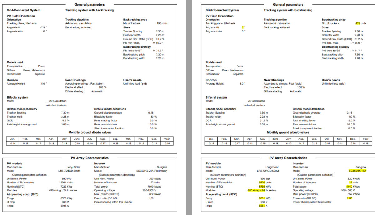
Hi Michele, thank you for your answer. Below you can find the comparison between the "General parameters" pages for the two projects. As for the question about irradiance optimization, I just checked it and it has not been activated in neither of the two simulations. I will also share my projects with you through the mail you have mentioned. Looking forward to having a clearer view on this matter 🙂
-
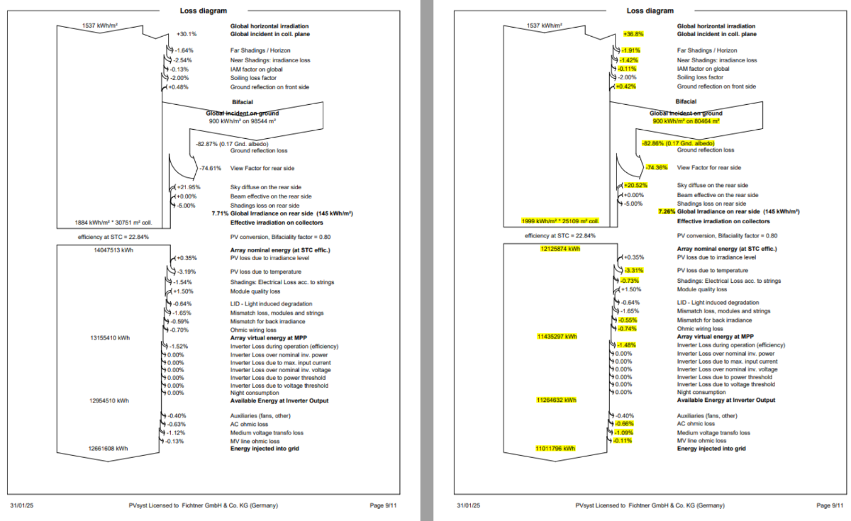
Hi everyone, for two neighboring projects having the same meteo data as well as same tracker configuration in terms of width and length of the tables, I get very different specific production in the order of 120 kWh/kWp. Looking at the loss diagrams of the two simulations, I noticed that the difference mainly relies upon the imported 3D scene (.pvc), as the one with lower production features a more undulating topography. Therefore, as far as I understood, it is reasonable to have higher losses such as Near shadings and shading losses according to strings for the project with challenging terrain. However, I was also noticing that the parameter Global Incindent in collec. plane is quite different, with the project with more challenging topography having a gain 6% less than the other. Such divergence can be justified by the different 3D scene? Considering all these aspects and seeing the below loss diagrams, do you think that for two close projects, such deviation in production can be linked to the 3D scene, meaning the underneath topography? I hope you can help me with those questions, and I'm available for further discussions. Best regards.