Rafael Santos

Continuing the question: I am thinking about 1 - ignoring this shape difference and count it as uncertainty, or 2 - Consider the module as monofacial, and "boost" GPOA values with the mantioned formula: E_Total = E_POA + E_Rear * 𝜑 or E_rear = RPOA * (1 - "Structural shading factor") The second option makes sense? If so, which formula would be more accurate? Thanks! Rafael

That's a very interesting topic! I am also carrying out a performance analysis, with RPOA measurement... Since it is not possible to use it on the .MET file (like GPOA), I am trying to fit the bifacial parameters (structure shading + transparent fraction) running multiple simulations and comparing the results (GlobBak) to the measured GPOA, to see which one fits best. Apart from the absolute values, all simulations showed the shape curve similar to GHI, while the measured curve showed a shape similar do GPOA: Is this have something to do with the assumption that the re-emitted irradiance is isotropic? This text below was taken from PVsyst help: Or am I doing something incorrect? Maybe "Globak" is not the right variable to compare with RPOA? Even so, would the shape of the curves would be that different? Best regards, Rafael

Hi, I am trying to run a stand alone project, but when I choose a bifacial module, the bifacial feature does not seem to show... Isn't it possible to simulate bifacial modules in stand alone projects? If it is not possible, is there a workaround to this? Beste regards, Rafael

Hi, Normally what I do in this case is to use LID=0,6% (wich is 1% warranted at the end of the first year - 0,4% degradation at the end of the year).

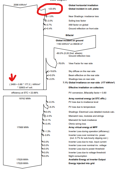
Hi! I am currently working on a project with 1-year on site measurements, with 10 minute temporal resolution. I want to predict the annual energy production (using TMY), but the data from TMY is hourly based. I thought at first of simulating with 3 MET inputs: 1-year measurement (hourly), 1-year measurement (10-minutes), and TMY (hourly), and then apply the correction: SIM_TMY_corrected = (SIM_10-min_meas / SIM_hourly_meas) * SIM_TMY_hourly I thought this would have been a fair approximation, as the sub-hourly simulation would only have an effect on the clipping losses. But as I made the simulations, I noticed that the sub-hourly simulation has a very large effect also on the transposition gain, as showed below: Hourly measurements: 10-Minute measurements: With that being said, ,y question is: would still make sense to apply the correction above? In this particular case: CF = 17529 MWh / 17389 MWh Best regards, Rafael

I just uploaded a .MET file containing clear sky radiation data instead of regular GHI, and ran a batch simulation changing azimuth angles, and the optimal azimuth angle was 0deg N, as expected! So, the "problem" here is specifically the TMY. Altough at "normal" conditions (considering only the universe geometry) the optimal azimuth should be zero, some sites have specific climatology (tend to be cloudier at mornings or afternoons on certain months), and this may affect the optimal annual energy production, specially considering fixed-tilt modules.

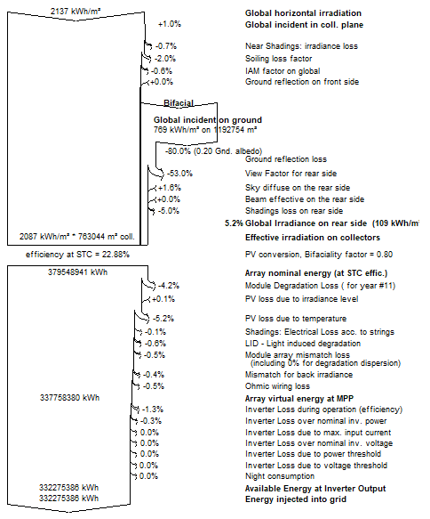
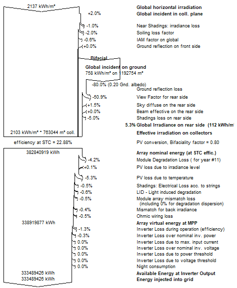
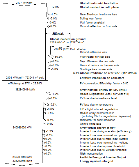
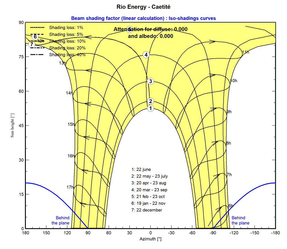
Thanks for the reply! I performed another simulation with electrical shading losses (acc. to module strings, 100% fraction for electrical effect). Although the results are slightly different, the question remais, as I am still getting higher results for a 40° azimuth: Azimuth: 0° Azimuth: 40° The main concern here is not the shading or any other losses, but the second line: "Global incident on coll. plane". This gain should be higher for a 0° azimuth. Best regards, Rafael

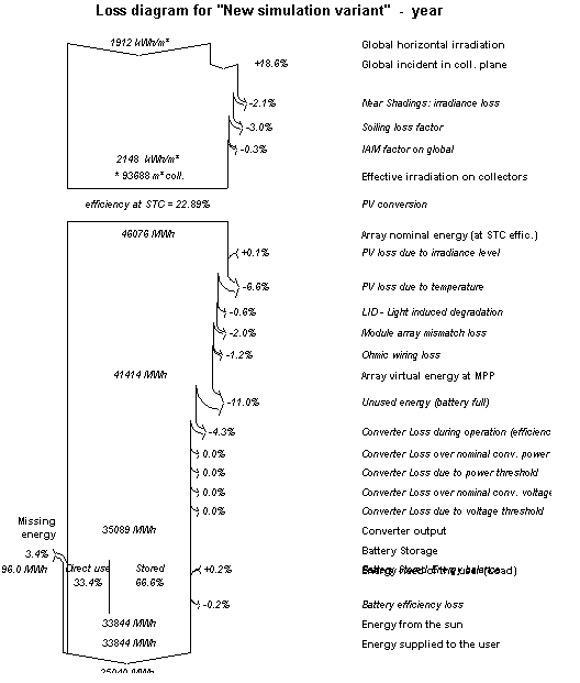
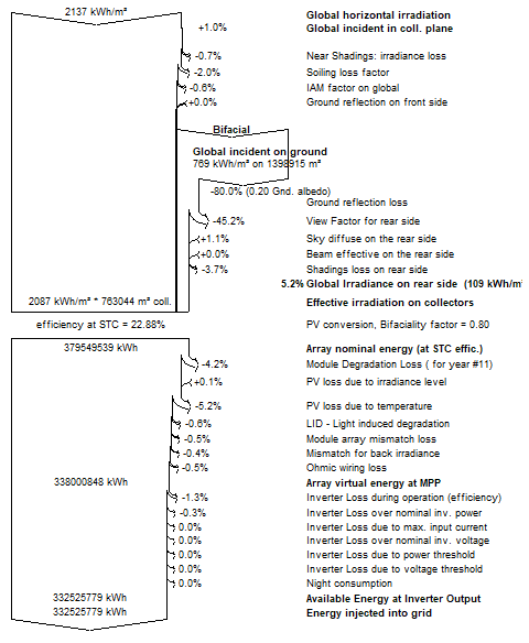
Hi, I performed simulations with different azimuth angles (-10 to 90 degrees, in 5-degrees steps) and surprisingly I got higher annual energy production with most of the azimuth angles that are different than zero (the project is located on the southern hemisphere). Simulation with Azimuth=0°: Simulation with Azimuth=40°: Intuitively, I would think a 0° azimuth would always give me the higher energy yield, which apparently is not so... Of course, the configuration is exactly the same, except for the azimuth. The modules are fixed, tilted 12°, and bifacial. Best regards, Rafael

Hi, Since I updated to version 7.2.3 the iso-shadings curves is showing the "behind the plane" blue line. I thought this was only for fixed planes, but I am using trackers with backtracking (see picture attached). Is this a bug or did I misundertand something? Best regards, Rafael

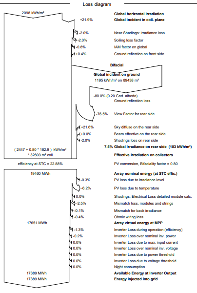
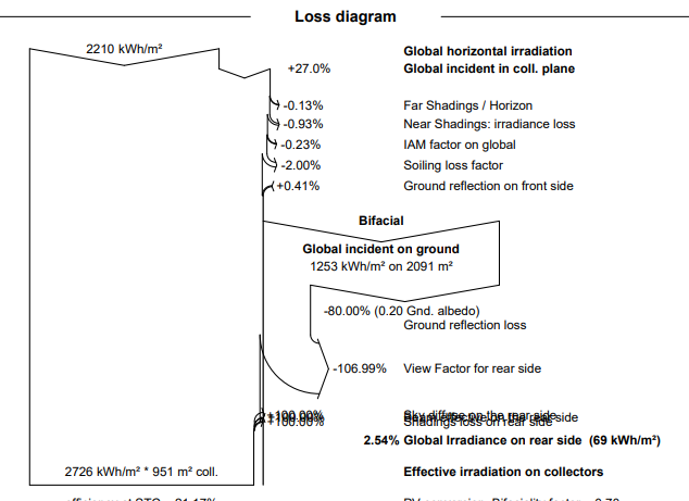
Hi, I upgraded to version 7,2 and found problems simulating with bifacial modules. I am having a few unrealistic values (e.g. View factor of more than 100%), I attached a image of the loss diagram. Finally, I downgraded to the previous version (7.1.8) and the results were fine!

Updating: I did some reverse engineering, and found that with the loss value of 115.95 kWh/m² (36.36%) everything work fine, including all the other losses! Maybe there is something wrong with the values on the "View Factor for Rear Side" losses presented on the table? Regards, Rafael

Growth of mismatch is also included! =)

Regarding the RMS dispersion values, this is strange, because I allways set them zero and it works just fine...

Hi, By default, PVsyst considers the average degradation loss throught the whole year. So, if you put degradation loss of 0,4%/year, for year 1, it will consider degratadion losses of 0,2% (starting the year with no degradation losses at all, since the modules are brand new, and ending the year with 0,4% losses, thus averaging 0,2%). Year 0 means it will not consider any degradation losses. So if want to make a batch simulation for eg. 10 years and you use 1 to 10, PVsyst will consider the average losses throught each year. If you want to change for the losses in the beggining of each year, you should use 0 to 9. Best regards, Rafael

Hi, I recentrly ran a simulation using a bi-facial module, and I was trying to understand better the physics and results of it. I came across a loss value of -78,82% for the parameter "View Factor for Rear Side" as shown in the loss diagram attached. My question is how It came to this number, since my absolute results were: - Global incident on ground: 1581 kWh/m²; - Ground reflexion loss: 1265 kWh/m² (this value is ok, 80% loss due to an albedo of 0.2); - View Factor for the rear side: 749 kWh/m² (this is strange, because I understand it is supposed to be (1581-1265)*0.7882) Is it something I am doing wrong? Best regards, Rafael Loss Results Loss Diagram