S.Faulkner

It appears that PVsyst calculates the effective rear mismatch loss by applying the loss (eg 10%) to the rear irradiance BEFORE the bifacial factor is applied, whereas Help says that it is applied after the bifacial factor, ie 10% x GlobBakEn / (GlobBakEn + GlobEff). Actually, from reverse-calculation it looks like it is applied to GlobBak / (GlobBakEn + GlobEff)? I have only checked this with V6.88, not V7. See https://forum.pvsyst.com/viewtopic.php?f=25&t=4992#p11241

It appears that PVsyst actually calculates the effective rear mismatch loss by applying the loss (10%) to the rear irradiance BEFORE the bifacial factor is applied, ie in your example: = 10% x [38/(38+1742)] =0.213% It makes sense that the mismatch loss, being an electrical effect within the module, should logically be applied after applying the bifacial factor of 0.7. However, we should also note that "The default of 10% is just a rough estimation". If the loss is applied after the bifacial factor, then a loss of about 14.4% (varying slightly with amount of bifacial uplift) will give the same result.

Thanks for explaining this, but I don't understand. You seem to be saying that the drop in efficiency is because inverter is more often operating at a lower power, but the difference is very small and the change in efficiency near maximum power doesn't vary much at all. In the case below, the grid limitation is only a few percent below the inverter maximum output, not enough to change the efficiency. Do you mean that changing the IV setpoint to achieve the grid limitation puts the inverter into a lower efficiency operating range? My feeling is that this isn't useful, and I wonder if others agree. I would like to know the efficiency that is achievable by the inverter without grid limitation, and then the loss that occurs as a result of the grid limitation. But is the assessment done this way so that the effects of the curtailment method are taken into account, such as voltage or current going outside of the inverter's allowable range?

I've noticed that in 6.47, setting a grid power limitation affects the inverter efficiency loss, as well as the Inverter over nom. power (clipping loss). The combined loss seems to be correct (see below), but is it correct that the efficiency changes? I noticed this when I calculated results with and without the grid limitation, so that I could find out how much of the clipping occurs at the inverter and how much at the grid injection point (this affects optimization of the inverter quantities). Case 1 Without grid limitation: Inverter Loss during operation (efficiency) -1.68% Inverter over nom. power (clipping loss) -0.91% Case 2 With grid limitation: Inverter Loss during operation (efficiency) -2.12% Inverter over nom. power (clipping loss) -1.36% The inverter Euro efficiency is 98.35% so the loss should be around 1.65%, ie the efficiency loss for case 1 (without the grid limitation) looks correct. I exported the hourly data for each case, and found that if I apply the grid limit in a spreadsheet (apply a cap to E_grid) the additional loss is -0.88%. Combining this with the efficiency and clipping loss for case 1 gives a total loss of -3.44%, and the total for case 2 is -3.46%, ie the total loss appears to be correct. (I previously added this comment on the end of the Grid Power Limitation post but I thought may be better to raise it as a new topic)

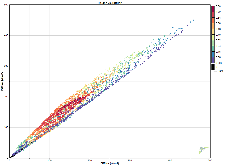
Revised question I understand that for transposition the diffuse irradiance is split into circumsolar and isotropic (and horizon) components and the circumsolar is treated like the direct irradiance in the transposition. I had previously assumed that the circumsolar component was actually subtracted from the diffuse irradiance and added to the direct irradiance, and therefore treated like direct irradiance for all the subsequent calculations. I gather from the data* that this isn't done, and that PVsyst therefore treats the circumsolar component as diffuse for all subsequent calculations (reflection and shading being affected in particular). Is that correct, and is there any particular reason for not treating circumsolar the same as direct in subsequent calculations? * In PVsyst the diffuse irradiance generally increases from horizontal to plane of array. The isotropic component decreases as a result of some being behind the array, and the circumsolar component is (generally) increased in the same way as the direct irradiance. The circumsolar component must therefore be still included in the diffuse irradiance. Diffuse on POA vs Diffuse on horizontal, Perez, colour-coded by Kn (red is high, Blue is low)

I would like to see how much effect the synthesis of hourly data has on the results (for a large grid-connected tracking system, in particular the inverter clipping loss), so I tried producing multiple hourly datasets from the same monthly data. I used "Synthetic hourly data generation" under Databases, changed the file name and reran the synthesis (Execute Generation) multiple times. However the resulting .met files all were the same. Confirmed by exporting to csv files. How can I get the synthesis to run again to produce different .met file results? I'm using V6.39. Help says "Please note that this generation is a fully random process: two successive generations performed from the same monthly data will result in completely different years."

My understanding is that clouds cause a blue-shift which has a small effect on c-Si modules, but low sun causes a red-shift that has an opposite effect. And therefore these balance to some extent. Is that right? Some consideration of these would be nice to have, but nowhere as nice to have as sub-hourly processing, in my humble opinion.

I'm sorry but I still don't understand why there isn't electrical loss for diffuse shading. Doesn't the amount of diffuse shading vary with position on the module? Does the electrical effect not apply to small differences in irradiance (such as diffuse) in the way that is does to large (shading of beam irradiance)? As I understand it, the diffuse shading (after taking account of irradiance behind the POA) varies from zero at the top of the array to a maximum at the bottom, related to the angle above the horizon of the next array that is causing the shading, ie how much of the sky is blocked by the next array. At the top this angle is zero, and increases towards the bottom. If I have read the descriptions correctly, PVsyst calculates the diffuse shading loss as an integral of this varying shading? As an example, for array "height" 1.976m (one module in portrait), pitch 3m, tilted at 30deg. Diffuse shading factor (excluding loss due to sky behind POA) is 1 at the top, 0.74 at the bottom, and the average across the array is 0.91. If the module performance is determined by the cell with lowest irradiance (electrical effect), then the shading factor for diffuse-irradiance is 0.91 and for diffuse-electrical is 0.81 (0.74/0.91). As noted earlier this make a difference of roughly 1% to the overall result, which just meets my threshold for being worth assessing.

It appears that there is no shading electrical loss for diffuse irradiance, and I am wondering why? I noticed this when modelling a large tracking system with backtracking ie no shading of the beam component, which gives an irradiance loss of about 1% but zero electrical loss (According to module strings, 100% electrical effect). I set albedo to zero so that there is no related loss to confuse matters, ie the irradiance loss is entirely diffuse. I think I have set it up correctly but this lack of electrical loss makes me wonder. I'm expecting the electrical loss in this case to be roughly 1%. If I understand correctly, it should be at least as large as the irradiance loss, and can't be zero since the cells at the lowest point on the module see a smaller portion of the sky than the higher up cells. If I turn off backtracking there is as expected more irradiance loss (beam as well as diffuse) and an electrical loss that is larger than the irradiance loss, apparently coming only from shading of beam irradiance. As a check with no backtracking, I set the horizon very high so all the beam irradiance is blocked, and got a similar result - some irradiance shading loss but no associated electrical shading loss. So, what could be stopping the electrical loss, is this incorrect, or have I misunderstood something? (I have used 100% electrical effect and calculated According to modules strings)

I think I've answered this myself. I see now that a 3D scene is required, and that it is not too hard to set up since the number of trackers can be entered. The limit of 400 means I can only model one inverter but I can easy scale the results. The problem I now have is that there isn't any electrical shading loss, but I'll add to another post on that.

Am I right in understanding that in 6.39 when the power limitation is applied at the grid injection point, the loss is still shown as part of the Inverter Loss (over nominal inv. power)? This combined loss does drop as expected when changing from limitation applied at inverter to limitation applied at grid injection point.

Is it possible to set up near (self) shading calculation for a single-axis tracking system, without setting up a 3D shading scene? In other words like "unlimited sheds" for fixed tilt. I am modelling a large system (tens of MW) and I am not familiar with setting up 3D scenes. I could set up just one 1MW block but it would still be a lot of trackers. What is the easiest way to model the irradiance and electrical shading loss for a single axis tracking system with backtracking?